Lab 6 NHST and One-sample t-tests
6.1 Overview
In the previous chapters we have talked a lot about probability, comparing values across groups, and the inference from a sample to a population. In effect this is the essence of a lot of quantitative research that uses Null Hypothesis Significance Testing (NHST). You collect a sample, calculate a summary statistic about that sample, and use probability to establish the likelihood of that statistic occurring given certain situations.
However these concepts and ideas are hard to grasp at first and take playing around with data a few times to help get a better understanding of them. As such, to demonstrate these ideas further, and to start introducing commonly used tests and approaches to reproducible science, we will look at data related to sleep - a very important practice for the consolidation of learning that most of us do not get enough of! The study we will look at, to explore NHST more, is by one of our team and makes use of a well known task in Psychology, the Posner Paradigm: Woods et al (2009) The clock as a focus of selective attention in those with primary insomnia: An experimental study using a modified Posner paradigm .
In Chapter 6, through the activities, we will:
- Recap on testing a hypothesis through null hypothesis significance testing (NHST).
- Learn about approaches to reproducible experiments.
- Learn about binomial tests, as well as one-sample and independent t-tests.
- Learn about Posner paradigms and attention (PreClass), and the recency effect (InClass).
You don't need to read this to complete the activities it might help it make more sense.
The Posner paradigm (Posner, 1980), or the Posner Cueing task, is an attentional shift task, often used in a variety of fields to test spatial attention and how this is impacted by disorders or injury. It works by having participants look at a fixation cross in the center of a screen. To either side is an empty box. After a short delay, a cue (e.g. an arrow, an asterisk, or some other attention grabbing image) appears in one of the boxes (e.g. the box to the left of the fixation). This stays on screen for a few hundred milliseconds and is then replaced by a second image called the target (e.g. a different shape or image). Participants then have to respond left or right depending on which side of the fixation the target appeared. The dependent variable (DV) is the time taken to respond to the target appearing.
Key to the task is that in most trials the target will appear on the same side as the cue - the cue facilitates the target - and so participants will be quicker to respond. These are called valid trials. However, on some occasions the target will appear on the other side from the cue - e.g. the cue is on the left but the target appears on the right - and these are called invalid trials; participants will be slower to respond here as the cue misleads the participant.
From that, you should be starting to get an idea of how a Posner paradigm can help to measure attention and how it can help determine if people have issues in shifting attention (particularly from the invalid trials).
Reference:
Posner, M. (1980) Orienting of attention. Quarterly Journal of Experimental Psychology, 32(1), 3-25
6.2 PreClass Activity
ManyLabs - an approach to reproducible science
As you will learn from reading papers around the reproduciblity crisis, findings from experiments tend to be more reproducible when we increase participant numbers as this increases the power of the study's design; the likelihood of an experimental design detecting an effect, of a given size, when there is an effect to detect.
Power is a rather tricky concept in research that essentially amounts to the probability of your design being able to detect a significant difference when there is actually a significant difference to detect.
Power is an interplay between three other aspects of research design:
- alpha - your critical p-value (normally .05);
- the sample size (n);
- the effect size - how big is the difference (measured in a number of ways).
If you know any three of these four elements (power, alpha, effect size, n) you can calculate the fourth. We will save further discussion of power until Chapter 8 but if you want to read ahead then this blog is highly recommended: The Power Dialogues.
However, running several hundred participants in your one study can be a significant time and financial investment. Fortunately, the idea of a "ManyLabs" project can solve this problem. In this scenario the same experiment is run in various locations, all using the same procedure, and then the data is collapsed together and analysed as one. You can see a nice example of a Many Labs project in the paper Investigating Variation in Replicability (Klein et al., 2014). See how many labs and researchers are involved? Perhaps this is a better approach than lots of researchers working individually?
You think this all sounds a great idea so in your quest to be a collaborative reproducible researcher, and as a high-five to #TeamScience, you have joined a ManyLabs study replicating the findings of Woods et al. (2009). And that study is the premis for today's activities so let's start by having a quick-run through of the background of the experiment.
The Background
Woods and colleagues (2009) were interested in how the attention of people with poor sleep (Primary Insomnia - PI) was more tuned towards sleep-related stimuli than the attention of people with normal sleep (NS). Woods et al., hypothesised that participants with poor sleep would be more attentive to images related to a lack of sleep (i.e. an alarm clock showing 2AM) than participants with normal sleep would be. To test their hypothesis, the authors used a modified Posner paradigm, shown in Figure 1 of the paper, where images of an alarm clock acted as the cue on both valid and invalid trials, with the symbol ( .. ) being the target.
As can be seen in Figure 3 of Woods et al., the authors found that, on valid trials, whilst Primary Insomnia participants were faster in responding to the target, suggesting a slight increase in attention to the sleep related cue compared to the Normal Sleepers, there was no difference between groups. In contrast, for invalid trials, where poor sleep participants were expected to be distracted by the cue, the authors did indeed find a significant difference between groups consistent with their alternative hypothesis \(H_{1}\). Woods et al., concluded that poor sleepers (Primary Insomnia participants) were slower to respond to the target on invalid trials, compared to Normal Sleepers, due to the attention of the Primary Insomnia participants being drawn to the misleading cue (the alarm clock) on the invalid trials. This increased attention to the sleep-related cue led to an overall slower reponse to the target on these invalid trials.
As we said above, your lab is now part of a ManyLabs project that is looking to replicate this finding from Woods et al., (2009). As a pilot study, to test recruitment procedures, as well as the experimental paradigm and analyses pipeline, each lab gathers data from 22 Normal Sleepers. It is common to use only the control participants in a pilot (in this cas the NS participants) as they are more plentiful in the population than the experimental group (in this case PI participants) and saves using participants from the PI group which may be harder to obtain in the long run.
After gathering your data, we want to check the recruitment process and whether or not you have been able to draw a sample of normal sleepers similar to the sample drawn by Woods et al. To keep things straightforward, allowing us to understand the analyses better, we will only look at valid trials today, in NS participants, but in effect you could perform this test on all groups and conditions.
Are These Participants Normal Sleepers (NS)?
Below is the data from the 22 participants you have collected in your pilot study. Their mean reaction time for valid trials (in milliseconds) is shown in the right hand column, valid_rt.
| participant | valid_rt |
|---|---|
| 1 | 631.2 |
| 2 | 800.8 |
| 3 | 595.4 |
| 4 | 502.6 |
| 5 | 604.5 |
| 6 | 516.9 |
| 7 | 658.0 |
| 8 | 502.0 |
| 9 | 496.7 |
| 10 | 600.3 |
| 11 | 714.6 |
| 12 | 623.7 |
| 13 | 634.5 |
| 14 | 724.9 |
| 15 | 815.7 |
| 16 | 456.9 |
| 17 | 703.4 |
| 18 | 647.5 |
| 19 | 657.9 |
| 20 | 613.2 |
| 21 | 585.4 |
| 22 | 674.1 |
If you look at Woods et al (2009) Figure 3 you will see that, on valid trials, the mean reaction time for NS participants was 590 ms with a SD = 94 ms. As above, as part of our pilot study, we want to confirm that the 22 participants we have gathered are indeed Normal Sleepers. We will use the mean and SD from Woods et al., to confirm this. Essentially we are asking if the participants in the pilot are responding in a similar fashion as NS participants in the original study.
You will know from Chapter 5 that when using Null Hypothesis Significance Testing (NHST) we are working with both a null hypothesis (\(H_{0}\)) and an alternative hypothesis (\(H_{1}\)). Thinking about this study it makes some logical sense to think about it in terms of the null hypothesis (\(\mu1 = \mu2\)). So we could phrase our hypothesis as, "we hypothesise that there is no significant difference in mean reaction times to valid trials on the modified Posner experiment between the participants in the pilot study and the participants in the original study by Woods et al."
There is actually a few analytical ways to test our null hypothesis. Today we will show you how to do two of these. In tasks 1-3 we will use a binomial test and in tasks 4-8 we will use a one-sample t-test
The Binomial test is a very simple test that converts all participants to either being above or below a cut-off point, e.g. a mean value, and looking at the probability of finding that number of participants above that cut-off.
The one-sample t-test is similar in that it compares participants to a cut-off but it compares the mean and standard deviation of the collected sample to an ideal mean and standard deviation. By comparing the difference in means, divided by the standard deviation of the difference (a measure of the variance), we can determine if the sample is similar or not to the ideal mean.
6.2.1 The Binomial Test
The Binomial test is one of the most "basic tests" in null hypothesis testing in that it uses very little information. The binomial test is used when a study has two possible outcomes (success or failure) and you have an idea about what the probability of success is. This will sound familiar from the work we did in Chapter 4 and the Binomial distribution.
A binomial test tests if an observed result is different from what was expected. For example, is the number of heads in a series of coin flips different from what was expected. Or in our case for this chapter, we want to test whether our normal sleepers are giving reaction times that are the same or different from those measured by Woods et al. The following tasks will take you through the process.
6.2.2 Task 1: Creating a Dataframe
First we need to create a tibble with our data so that we can work with it.
- Enter the data for the 22 participants displayed above into a tibble and store it in
ns_data. Have one column showing the participant number (calledparticipant) and another column showing the mean reaction time, calledvalid_rt.- We saw how to enter data into tibbles in Chapter 5 PreClass Skill 3.
- You could type each value out or copy and paste them from the hint below.
You can use this code structure and replace the NULL values:
ns_data <- tibble(participant = c(NULL,NULL,...), valid_rt = c(NULL,NULL,...))
The values are: 631.2, 800.8, 595.4, 502.6, 604.5, 516.9, 658.0, 502.0, 496.7, 600.3, 714.6, 623.7, 634.5, 724.9, 815.7, 456.9, 703.4, 647.5, 657.9, 613.2, 585.4, 674.1
6.2.3 Task 2: Comparing Original and New Sample Reaction Times
Our next step is to establish how many participants from our pilot study are above the mean in the original study by Woods et al.
- In the original study the mean reaction time for valid trials was 590 ms. Store this value in
woods_mean.
- Now write code to calculate the number of participants in the new sample (
ns_datacreated in Task 1) that had a mean reaction time greater than the original paper's mean. Store this single value inn_participants.- The function
nrow()may help here. nrow()is similar tocount()orn()butnrow()returns the number as a single value and not in a tibble.- Be sure whatever method you use you end up with a single value, not a tibble. You may need to use
pull()orpluck()
- The function
Part 1
woods_mean <- value
Part 2
- A few ways to achieve this. Here are a couple you could try
ns_data %>% filter(x ? y) %>% count() %>% pull(?)
or
ns_data %>% filter(x ? y) %>% summarise(n = ?) %>% pull(?)
or
ns_data %>% filter(x ? y) %>% nrow()
or
dim[] %>% pluck()
Quickfire Questions
- The number of participants that have a mean reaction time for valid trials greater than that of the original paper is:
6.2.4 Task 3: Calculating Probability
Our final step for the binomial test is to compare our value from Task 2, 16 participants, to our hypothetical cut-off. We will work under the assumption that the mean reaction time from the original paper, i.e. 590 ms, is a good estimate for the population of good sleepers (NS). If that is true then each new participant that we have tested should have a .5 chance of being above this mean reaction time (\(p = .5\) for each participant).
To phrase this another way, the expected number of participants above the cut-off would be \(.5 \times N\), where \(N\) is the number of participants, or \(.5 \times 22\) = 11 participants.
- Calculate what would be the probability of observing at least 16 participants out of your 22 participants that had a
valid_rtgreater than the Woods et al (2009) mean value.- hint: We looked at very similar questions in Chapter 4 using
dbinom()andpbinom() - hint: The key thing is that you are asking about obtaining X or more successes. You will need to think back about cut-offs and
lower.tails.
- hint: We looked at very similar questions in Chapter 4 using
Think back to Chapter 4 where we used the binomial distribution. This question can be phrased as, what is the probability of obtaining X or more succeses out of Y trials, given the expected probability of Z.
- How many Xs? (see question)
- How many Ys? (see question)
- What is the probability of being either above or below the mean/cut-off? (see question)
-
You can use a dbinom() %>% sum() for this or maybe a
pbinom()
Quickfire Questions
- Using the Psychology standard \(\alpha = .05\), do you think these NS participants are responding in a similar fashion as the participants in the original paper? Select the appropriate answer:
- According to the Binomial test would you accept or reject the null hypothesis that we set at the start of this test?
The probability of obtaining 16 participants with a mean reaction time greater than the cut-off of 590 ms is p = .026. This is smaller than the field norm of p = .05. As such we can say that, using the binomial test, the new sample appears to be significantly different from the old sample as there is a significantly larger number of participants above the cut-off (M = 590ms) than would be expected if the new sample and the old sample were responding in a similar fashion. We would therefore reject our null hypothesis!
6.2.5 The One-Sample t-test
In Task 3 you ran a binomial test of the null hypothesis testing that here was no significant difference in mean reaction times to valid trials on the modified Posner experiment between the participants in the pilot study and the participants in the original study by Woods et al. However, the binomial test did not use all the available information in the data because each participant was simply classified as being above or below the mean of the original paper, i.e. yes or no. Information about the magnitude of the discrepancy from the mean was discarded. This information is really interesting and important however and if we wanted to maintain that information then we would need to use a one-sample \(t\)-test.
In a one-sample \(t\)-test, you test the null hypothesis \(H_0: \mu = \mu_0\) where:
- \(H_0\) is the symbol for the null hypothesis,
- \(\mu\) (pronounced mu - like few with an m) is the unobserved population mean,
- and \(\mu_0\) (mu-zero) is some other mean to compare against (which could be an alternative population or sample mean or a constant).
And we will do this by calculating the test statistic \(t\) which comes from the \(t\) distribution - more on that distribution below and in the lectures. The formula to calculate the observed test statistic \(t\) for the one-sample \(t\)-test is:
\[t = \frac{\mu - \mu_0}{s\ / \sqrt(n)}\]
- \(s\) is the stanard deviation of the sample collected,
- and \(n\) is the number of participants in the sample.
The eagle-eyed of you may have spotted that in Chapter 5 the null hypothesis was stated as:
\[H_0: \mu_1 = \mu_2\]
whereas in this Chapter we are stating it as:
\(S\)H_0: = _0$$
What's the difference? Conceptually there is no real difference. The null hypothesis in both situations is stating that there is no difference between the means. The only difference is that in Chapter 5 we know the actual mean of the groups of interest. In Chapter 6 we only really know the mean we want to compare against - \(\mu_0\). We do not know the actual mean of the population of interest (we only know the sample we have collected) - so this is written as \(\mu\).
Main thing to recognise is that the null hypothesis \(H_0\) always states that there is no significant difference between thw two means of interest - i.e. the two means are equivalent.
For the current problem:
- \(\mu\) is the unobserved true mean of all possible participants. We don't know this value. Our best guess is the mean of the sample of 22 participants so we will use that mean here. As such will substitute this value into our formula, which we call \(\bar{X}\) (pronounced X-bar), instead of \(\mu\)
- \(\mu_0\) is the mean to compare against. For us this is the mean of the original paper which we observed to be 590 ms.
So in other words we are testing the null hypothesis that \(H_0: \bar{X} =\) 590.
As such the formula for our one-sample \(t\)-test becomes:
\[t = \frac{\bar{X} - \mu_0}{s\ / \sqrt(n)}\]
Now we just need to fill in the numbers.
6.2.6 Task 4: Calculating the Mean and Standard Deviation
- Calculate the mean and standard deviation of
valid_rtfor our 22 participants (i.e., for all participant data at the top of this lab). - Store the mean in
ns_data_meanand store the standard deviation inns_data_sd. Make sure to store them both as single values!
In the below code, replace NULL with the code that would find the mean, m, of ns_data.
ns_data_mean <- summarise(NULL) %>% pull(NULL)
Replace NULL with the code that would find the standard deviation, sd, of ns_data.
ns_data_sd <- summarise(NULL) %>% pull(NULL)
6.2.7 Task 5: Calculating the Observed Test Statistic
From Task 4, you found out that \(\bar{X}\), the sample mean, was 625.464 ms, and \(s\), the sample standard deviation, was 94.307 ms. Now, keeping in mind that \(n\) is the number of observations/participants in the sample, and \(\mu_0\) is the mean from Woods et al (2009):
- Use the one-sample t-test formula above to compute your observed test statistic. Store the answer in
t_obs. - E.g.
t_obs <- (x - y)/(s/sqrt(n))
Answering this question will help you in this task as you'll also need these numbers to substitute into the formula:
- The mean from Woods et al (2009) was , and the number of participants in our sample is: (type in numbers) .
- Remember the solutions at the end of the chapter if you are stuck. To check that you are correct without looking at the solutions though - the observed \(t\)-value in
t_obs, to two decimal places, is
Remember BODMAS and/or PEDMAS when given more than one operation to calculate. (i.e. Brackets/Parenthesis, Orders/Exponents, Division, Multiplication, Addition, Subtraction)
t_obs <- (sample mean - woods mean) / (sample standard deviation / square root of n)
6.2.8 Task 6: Comparing the Observed Test Statistic to the t-distribution using pt()
Now you need to compare t_obs to the t-distribution to determine how likely the observation (i.e. your test statistic) is under the null hypothesis of no difference. To do this you need to use the pt() function.
- Use the
pt()function to get the \(p\)-value for a two-tailed test with \(\alpha\) level set to .05. The test has \(n - 1\) degrees of freedom, where \(n\) is the number of observations contributing to the sample mean \(\bar{X}\). Store the \(p\) value in the variablepval.
- Do you reject the null?
- Hint: The
pt()function works similar topbinom()andpnorm(). - Hint: Because we want the p-value for a two-tailed test, multiply
pt()by two.
Remember to get help you can enter ?pt in the console.
The pt() function works similar to pbinom() and pnorm():
-
pval <- pt(test statistic, df, lower.tail = FALSE) * 2 - Use the absolute value of the test statistic; i.e. ignore minus signs.
-
Remember,
dfis equal ton-1. -
Use
lower.tail = FALSEbecause we are wanting to know the probability of obtaining a value higher than the one we got. - Reject the null at the field standard of p < .05
6.2.9 Task 7: Comparing the Observed Test Statistic to the t-distribution using t.test()
Now that you have done this by hand, try using the t.test() function to get the same result. Take a moment to read the documentation for this function by typing ?t.test in the console window. No need to store the t-test output in a dataframe but do check that the p-value matches the pval in Task 6.
- The structure of the
t.test()function ist.test(column_of_data, mu = mean_to_compare_against)
The function requires a vector, not a table, as the first argument. You can use the pull() function to pull out the valid_rt column from the tibble ns_data with pull(ns_data, valid_rt).
You also need to include mu in the t.test(), where mu is equal to the mean you are comparing to.
Quickfire Questions
To make sure you are understanding the output of the t-test, try to answer the following questions.
To three decimal places, type in the p value for the t-test in Task 7
As such this one sample t-test is
The outcome of the binomial test and the one sample t-test produce answer
6.2.10 Task 8: Drawing Conclusions about the new data
Given these results, what do you conclude about how similar these 22 participants are to the original participants in Woods et al (2009) and whether or not you have managed to recruit sleepers similar to that study?
- Think about which test used more of the available information?
- Also, how reliable is the finding if the two tests give different answers?
We have given some of our thoughts at the end of the chapter.
Job Done - Activity Complete!
That's all! There is quite a bit in this lab in terms of theory of Null Hypothesis Significance Testing (NHST) so you might want to go back and add any informative points to your Portfolio. Post any questions on the forums
6.3 InClass Activity
The PreClass activity looked at the situation where you had gathered one sample of data (from one group of participants) and you want to compare that one group to a known value, e.g. a standard value. An extension of this design is where you gather data from two samples. Two-sample designs are very common in Psychology as often we want to know whether there is a difference between groups on a particular variable. We looked at a similar idead in Chapter 5 where we did this comparison through simulation. Today we will look at through the \(t\)-test analysis introduced in Chapter 6
Comparing the Means of Two Samples
First thing to not is that there are different types of two-sample designs depending on whether or not the two groups are independent (e.g. different participants on different conditions) or not (e.g. same participants on different conditions). In today's exercise we will focus on independent samples, which typically means that the observations in the two groups are unrelated - usually meaning different people. In Chapter 7 you will examine cases where the observations in the two groups are from pairs (paired samples) - most often the same people but could also be a matched-pairs design.
Now that we are progressing through this book, we will start to reduce the pointers for things that you should make a note of. By now you should have a really good idea yourself about what you need to remember. That said, one of the really confusing things about research design is that there are many names for the same type of design. This is definitely something you should be writing out in your own words, to remember it better, if it is something you struggle with.
Here is a very brief summary:
- independent and between-subjects design typically mean the same thing - different participants in different conditions.
- within-subjects, dependent samples, paired samples, and repeated measures tend to mean the same participants in all conditions
- matched-pairs design means different people in different conditions but you have matched participants across the conditions so that they are effectively the same person (e.g. age, IQ, Social Economic Status, etc). These designs are analysed as though they were a within-subjects design.
- mixed design is when there is a combination of within-subjects and between-subjects designs in the one experiment. For example, say you are looking at attractiveness and dominance of male and female faces. Everyone might see both male and female faces (within) but half of the participants do ratings of attractiveness and half do ratings of trustworthiness (between).
- The paper we are looking at in this InClass activity technically uses a mixed design at times but we will use the between-subjects element to show you how to run independent t-tests.
Spend some time when reading articles to really figure out the design they are using.
Background
For this lab we will be revisiting the data from Schroeder and Epley (2015), which you first encountered as part of the homework for Chapter 5. You can take a look at the Psychological Science article here:
Schroeder, J. and Epley, N. (2015). The sound of intellect: Speech reveals a thoughtful mind, increasing a job candidate's appeal. Psychological Science, 26, 277--891.
The abstract from this article explains more about the different experiments conducted (we will be specifically looking at the dataset from Experiment 4, courtesy of the Open Stats Lab):
"A person's mental capacities, such as intellect, cannot be observed directly and so are instead inferred from indirect cues. We predicted that a person's intellect would be conveyed most strongly through a cue closely tied to actual thinking: his or her voice. Hypothetical employers (Experiments 1-3b) and professional recruiters (Experiment 4) watched, listened to, or read job candidates' pitches about why they should be hired. These evaluators (the employers) rated a candidate as more competent, thoughtful, and intelligent when they heard a pitch rather than read it and, as a result, had a more favorable impression of the candidate and were more interested in hiring the candidate. Adding voice to written pitches, by having trained actors (Experiment 3a) or untrained adults (Experiment 3b) read them, produced the same results. Adding visual cues to audio pitches did not alter evaluations of the candidates. For conveying one's intellect, it is important that one's voice, quite literally, be heard."
To recap on Experiment 4, 39 professional recruiters from Fortune 500 companies evaluated job pitches of M.B.A. candidates (Masters in Business Administration) from the University of Chicago Booth School of Business. The methods and results appear on pages 887--889 of the article if you want to look at them specifically for more details. The original data, in wide format, can be found at the Open Stats Lab website for later self-directed learning. Today however, we will be working with a modfied version in "tidy" format which can be downloaded from here. I you are unsure about tidy format, refer back to the inclass activities of Chapter 2.
Today's Goal!
The overall goal today is to learn about running a \(t\)-test on between-subjects data, as well as learning about analysing actual data along the way. As such, our task today is to reproduce a figure and the results from the article (p. 887-888). The two packages you will need are tidyverse, which we have used a lot, and broom, which is new to you but will become your friend. One of the main functions we use in broom is broom::tidy() - this is an incredibly useful function that converts the output of an inferential test in R from a combination of text and lists, that are really hard to work with - technically called objects - into a tibble that you are very familiar with and that you can then use much more easily. Might that be worth making a note of? We will show you how to use this function today and then ask you to use it over the coming chapters
If you are using the Boyd Orr labs, broom is already installed and just needs called to the library(). If you are using your own machine, you will need to install it one time to begin with if you have never installed it before.
6.3.1 Task 1: Evaluators
- Open a new script or R Markdown file and use code to call
broomandtidyverseinto your library.
Note: Order is important when calling multiple libraries - if two libraries have a function named the same thing, R will use the function from the library loaded in last. We recommend calling libraries in an order that tidyverse is called last as the functions in that library are used most often.
The file called
evaluators.csvcontains the demographics of the 39 raters. After downloading and unzipping the data, and of course setting the working directory, load in the information from this file and store it in a tibble calledevaluators.Now, use code to:
- calculate the overall mean and standard deviation of the age of the evaluators.
- count how many male and how many female evaluators were in the study.
Note: Probably easier doing this task in seperate lines of code. Remeber the solutions are at the end of the Chapter.
Note: there are NAs in the data so you will need to include a call to na.rm = TRUE.
- Remember to load the libraries you need!
- Also make sure you've downloaded and saved the data in the folder you're working from.
-
You can use
summarise()andcount()or a pipeline withgroup_by()to complete this task. - When analysing the number of male and female evaluators it isn't initially clear that '1' represents males and '2' represents females.
-
We can use
recode()to convert the numeric names to indicate something more meaningful. Have a look at?recodeto see if you can work out how to use it. It'll help to usemutate()to create a new variable torecode()the numeric names for evaluators. - This website is also incredibly useful and one to save for anytime you need to use recode(): https://debruine.github.io/posts/recode/
- For your own analysis and future reproducible analyses, it's a good idea to make these representations clearer to others.
Quickfire Questions
Fill in the below answers to check that your calculations are correct. Remember that the solutions are at the end of the chapter:
- What was the mean age of the evaluators in the study? Type in your answer to one decimal place:
- What was the standard deviation of the age of the evaluators in the study? Type in your answer to two decimal places:
- How many participants were noted as being female:
- How many participants were noted as being male:
Group Discussion Point
The paper claims that the mean age of the evaluators was 30.85 years (SD = 6.24) and that there were 9 male and 30 female evaluators. Do you agree? Why might there be differences?
This paper claimed there were 9 males, however looking at your results you can see only 4 males, with 5 NA entries making up the rest of the participant count. It looks like the NA and male entries have been combined! That information might not be clear to a person re-analysing the data.
This is why it's important to have reproducible data analyses for others to examine. Having another pair of eyes examining your data can be very beneficial in spotting any discrepancies - this allows for critical evaluation of analyses and results and improves the quality of research being published. All the more reason to emphasize the importance of conducting replication studies! #ReproducibleScience
6.3.2 Task 2: Ratings
We are now going to calculate an overall intellect rating given by each evaluator. To break that down a bit, we are going to calculate how intellectual the evaluators (the raters) thought candidates were overall, depending on whether or not the evaluators read or listened to the candidates' resume pitches. This is calculated by averaging the ratings of competent, thoughtful and intelligent for each evaluator held within ratings.csv.
Note: we are not looking at ratings to individual candidates; we are looking at overall ratings for each evaluator. This is a bit confusing but makes sense if you stop to think about it a little. You can think about it in terms of "do raters rate differently depending on whether they read or listen to a resume pitch".
We will then combine the overall intellect rating with the overall impression ratings and overall hire ratings for each evaluator, all ready found in ratings.csv. In the end we will have a new tibble - let's call it ratings2 - which has the below structure:
- eval_id shows the evaluator ID. Each evaluator has a different ID. So all the 1's are the same evaluator.
- Category shows the scale that they were rating on - intellect, hire, impression
- Rating shows the overall rating given by that evaluator on a given scale.
- condition shows whether that evaluater listened to (e.g. evaluators 1, 2 and 3), or read (e.g. evaluator 4) the resume.
| eval_id | Category | Rating | condition |
|---|---|---|---|
| 1 | hire | 6.000 | listened |
| 1 | impression | 7.000 | listened |
| 1 | intellect | 6.000 | listened |
| 2 | hire | 4.000 | listened |
| 2 | impression | 4.667 | listened |
| 2 | intellect | 5.667 | listened |
| 3 | hire | 5.000 | listened |
| 3 | impression | 8.333 | listened |
| 3 | intellect | 6.000 | listened |
| 4 | hire | 4.000 | read |
| 4 | impression | 4.667 | read |
| 4 | intellect | 3.333 | read |
The following steps describe how to create the above tibble but you might want to have a bash yourself without reading them first. The trick when doing data analysis and data wrangling is to first think about what you want to achieve - the end goal - and then what function do I need to use. You know what you want to end up with - the above table - now how do you get there?
Steps 1-3 calculate the new intellect rating. Steps 4 and 5 combine this rating to all other information.
Load the data found in
ratings.csvinto a tibble calledratings.filter()only the relevant variables (thoughtful, competent, intelligent) into a new tibble (call it what you like - in the solutions we useiratings), and calculate a meanRatingfor each evaluator.Add on a new column called
Categorywhere every entry is the wordintellect. This tells us that every number in this tibble is an intellect rating.Now create a new tibble called
ratings2and filter into it just the impression and hire ratings from the originalratingstibble. Next, bind this tibble with the tibble you created in step 3 to bring together the intellect, impression, and hire ratings, inratings2.Join
ratings2with theevaluatortibble that we created in Task 1. Keep only the necessary columns as shown above and arrange by Evaluator and Category.
Don't forget to use the hints below or the solution at the end of the Chapter if you are stuck. One thing to think about though is that the above steps don't help, again just go back to what you want to achieve and ask yourself how would you do that, and think backwards.
-
Make sure you've downloaded and saved the data into the folder you're working from.
-
filter(Category %in% c())might work and then usegroup_by()andsummarize()to calculate a meanRatingfor each evaluator. -
Use
mutate()to create a new column. -
bind_rows()from Chapter 2 will help you to combine these variables from two separate tibbles. -
Use
inner_join()with the common column in both tibbles.select()andarrange()will help you here too.
6.3.3 Task 3: Creating a Figure
To recap, we now have ratings2 which contains an overall Rating score for each evaluator on the three Category (within: hire, impression, intellect) depending on which condition that evaluator was in (between: listened or read). Great! Now we have all the information we need to replicate Figure 7 in the article (page 888), shown here:
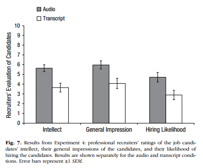
Figure 6.1: Figure 7 from Schroeder and Epley (2015) which you should try to replicate.
Replace the NULLs below to create a very basic version of this figure. You did something like this for the Chapter 5 assignment and again in the Chapter 3 Visualisation tasks.
group_means <- group_by(ratings2, NULL, NULL) %>%
  summarise(Rating = mean(Rating))

ggplot(group_means, aes(NULL, NULL, fill = NULL)) +
  geom_col(position = "dodge")
Group Discussion Point
Improve Your Figure: Discuss with others how you could improve this plot. What other geom_() options could you try? Are barcharts that informative or would something else be better? How would you add or change the labels of your plot? Could you change the colours in your figure?
Next, have a look at the possible solution below to see a modern way of presenting this information. There are some new functions in this solution that you should play about with to understand what they do. Remember it is a layering system, so remove lines and see what happens. Note how in the solution the Figure shows the raw data points as well as the means in each condition; this gives a better impression of the true data as just showing the means can be misleading. You can continue your further exploration of visualisations by reading this paper later when you have a chance: Weissberger et al., 2015, Beyond Bar and Line Graphs: Time for a New Data Presentation Paradigm
Filling in the code as below will create a basic figure as shown:
group_means <- ratings2 %>%
  group_by(condition, Category) %>%
  summarise(Rating = mean(Rating))
## `summarise()` has grouped output by 'condition'. You can override using the `.groups` argument.ggplot(group_means, aes(Category, Rating, fill = condition)) +
geom_col(position = "dodge")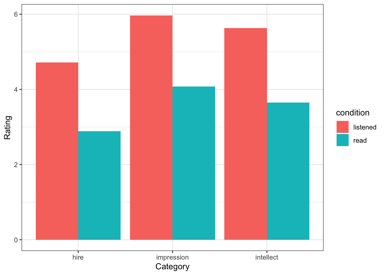
Figure 6.2: A basic solution to Figure 7
Or alternatively, for a more modern presentation of the data:
group_means <- ratings2 %>%
  group_by(condition, Category) %>%
  summarise(Rating = mean(Rating))
## `summarise()` has grouped output by 'condition'. You can override using the `.groups` argument.ggplot(ratings2, aes(condition, Rating, color = condition)) +
geom_jitter(alpha = .4) +
geom_violin(aes(fill = condition), alpha = .1) +
facet_wrap(~Category) +
geom_point(data = group_means, size = 2) +
labs(x = "Category", y = "Recruiters' Evaluation of Candidates") +
coord_cartesian(ylim = c(0, 10), expand = FALSE) +
guides(color = "none", fill = "none") +
theme_bw()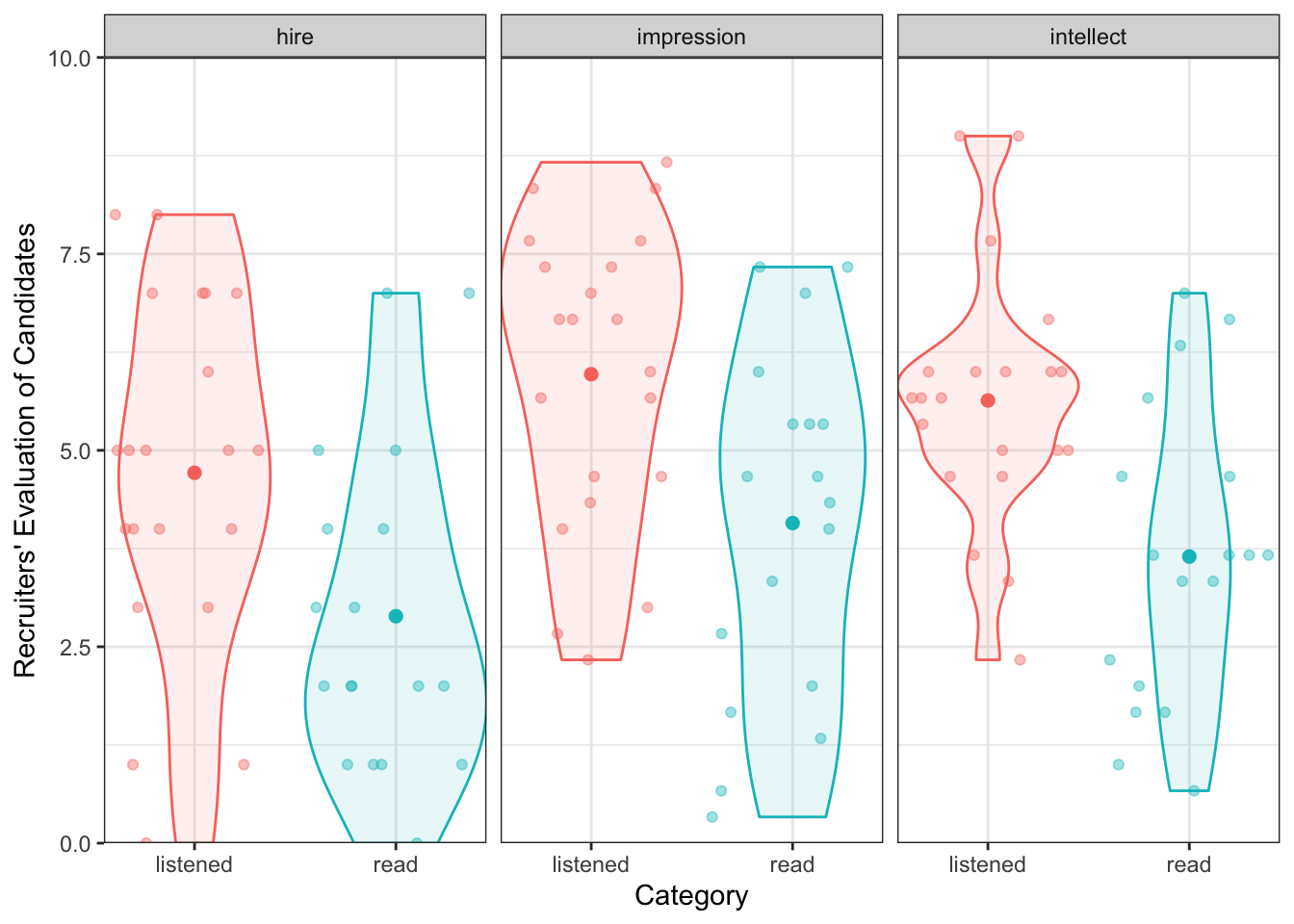
Figure 6.3: A possible alternative to Figure 7
6.3.4 Task 4: t-tests
Brilliant! So far we have checked the descriptives and the visualisations, and the last thing now is to check the inferential tests; the t-tests. You should still have ratings2 stored from Task 2. From this tibble, let's reproduce the t-test results from the article and at the same time show you how to run a t-test. You can refer back to the lectures to understand the maths a between-subjects t-test but essentially it is a measure between the difference in means over the variance about those means.
Here is a paragraph from the paper describing the results (p. 887):
"The pattern of evaluations by professional recruiters replicated the pattern observed in Experiments 1 through 3b (see Fig. 7). In particular, the recruiters believed that the job candidates had greater intellect---were more competent, thoughtful, and intelligent---when they listened to pitches (M = 5.63, SD = 1.61) than when they read pitches (M = 3.65, SD = 1.91), t(37) = 3.53, p < .01, 95% CI of the difference = [0.85, 3.13], d = 1.16. The recruiters also formed more positive impressions of the candidates---rated them as more likeable and had a more positive and less negative impression of them---when they listened to pitches (M = 5.97, SD = 1.92) than when they read pitches (M = 4.07, SD = 2.23), t(37) = 2.85, p < .01, 95% CI of the difference = [0.55, 3.24], d = 0.94. Finally, they also reported being more likely to hire the candidates when they listened to pitches (M = 4.71, SD = 2.26) than when they read the same pitches (M = 2.89, SD = 2.06), t(37) = 2.62, p < .01, 95% CI of the difference = [0.41, 3.24], d = 0.86."
We are going to run the t-tests for Intellect, Hire and Impression; each time comparing evaluators overall ratings for the listened group versus overall ratings for the read group to see if there was a significant difference between the two conditions: i.e. did the evaluators who listened to pitches give a significant higher or lower rating than evaluators that read pitches.
In terms of hypotheses, we could phrase the null hypothesis for this tests as there is no significant difference between overall ratings on the {insert trait} scale between evaluators who listened to resume pitches and evaluatoris who read the resume pitches (\(H_0: \mu_1 = \mu2\)). Alternatively, we could state it as there will be a significant difference between overall ratings on the {insert trait} scale between evaluators who listened to resume pitches and evaluatoris who read the resume pitches (\(H_1: \mu_1 \ne \mu2\)).
Now would be a good time to add to your notes about what is the difference between a positive and negative value as the outcome to a t-test? Remember? It just tells you which group had the bigger mean - the absolute value will be the same. Most commonly, t-tests are reported as a positive value.
To clarify, we are going to run three between-subjects t-tests in total; one for intellect ratings; one for hire ratings; one for impression ratings. We will show you how to run the t-test on intellect ratings and then ask you to do the remaining two t-tests yourself.
To run this analysis on the intellect ratings you will need the function t.test() and you will use broom::tidy() to pull out the results from each t-test into a tibble Below, we show you how to create the group means and then run the t-test for intellect. Run these lines and have a look at what they do.
- First we calculate the group means:
group_means <- ratings2 %>%
  group_by(condition, Category) %>%
  summarise(m = mean(Rating), sd = sd(Rating))
## `summarise()` has grouped output by 'condition'. You can override using the `.groups` argument.- And we can call them and look at them by typing:
group_means| condition | Category | m | sd |
|---|---|---|---|
| listened | hire | 4.714286 | 2.261479 |
| listened | impression | 5.968254 | 1.917477 |
| listened | intellect | 5.634921 | 1.608674 |
| read | hire | 2.888889 | 2.054805 |
| read | impression | 4.074074 | 2.233306 |
| read | intellect | 3.648148 | 1.911343 |
- Now to just look at intellect ratings we need to filter them into a new tibble:
intellect <- filter(ratings2, Category == "intellect")- And then we run the actual t-test and tidy it into a table.
t.test()requires two vectors as inputpull()will pull out a single column from a tibble, e.g. Rating from intellecttidy()takes information from a test and turns it into a tibble. Try running the t.test with and without piping intotidy()to see what it does differently.
intellect_t <- t.test(intellect %>%
                        filter(condition == "listened") %>%
                        pull(Rating),
                      intellect %>%
                        filter(condition == "read") %>%
                        pull(Rating),
                      var.equal = TRUE) %>%
  tidy()
Now lets look at the intellect_ttibble we have created (assuming you piped into tidy()):
| estimate | estimate1 | estimate2 | statistic | p.value | parameter | conf.low | conf.high | method | alternative |
|---|---|---|---|---|---|---|---|---|---|
| 1.987 | 5.635 | 3.648 | 3.526 | 0.001 | 37 | 0.845 | 3.128 | Two Sample t-test | two.sided |
From the resultant tibble, intellect_t, you can see that you ran a Two Sample t-test (meaning between-subjects) with a two-tailed hypothesis test ("two.sided"). The mean for the listened condition, estimate1, was 5.635, whilst the mean for the read condition, estimate2 was 3.648 - compare these to the means in group_means as a sanity check. So an overall the was a difference between the two means of 1.987. The degrees of freedom for the test, parameter, was 37. The observed t-value, statistic, was 3.526, and it was significant as the p-value, p.value, was p = 0.0011, which is lower than the field standard Type 1 error rate of \(\alpha = .05\).
As you will know from your lectures, a t-test is presented as t(df) = t-value, p = p-value. As such, this t-test would be written up as: t(37) = 3.526, p = 0.001.
Thinking about interpretation of this finding, as the effect was significant, we can reject the null hypothesis that there is no significant difference between mean ratings of those who listened to resumes and those who read the resumes, for intellect ratings. We can go further than that and say that the overall intellect ratings for those that listened to the resume was significantly higher (mean diff = 1.987) than those who read the resumes, t(37) = 3.526, p = 0.001, and as such we accept the alternative hypothesis. This would suggest that hearing people speak leads evaluators to rate the candidates as more intellectual than when you merely read the words they have written.
Now Try:
Running the remaining t-tests for
hireand forimpression. Store them in tibbles calledhire_tandimpress_trespectively.Bind the rows of
intellect_t,hire_tandimpress_tto create a table of the three t-tests calledresults. It should look like this:
| Category | estimate | estimate1 | estimate2 | statistic | p.value | parameter | conf.low | conf.high | method | alternative |
|---|---|---|---|---|---|---|---|---|---|---|
| intellect | 1.987 | 5.635 | 3.648 | 3.526 | 0.001 | 37 | 0.845 | 3.128 | Two Sample t-test | two.sided |
| hire | 1.825 | 4.714 | 2.889 | 2.620 | 0.013 | 37 | 0.414 | 3.237 | Two Sample t-test | two.sided |
| impression | 1.894 | 5.968 | 4.074 | 2.851 | 0.007 | 37 | 0.548 | 3.240 | Two Sample t-test | two.sided |
Quickfire Questions
Check your results for
hire. Enter the mean estimates and t-test results (means and t-value to 2 decimal places, p-value to 3 decimal places):Mean
estimate1(listened condition) =Mean
estimate2(read condition) =t() = , p =
Looking at this result, True or False, this result is significant at \(\alpha = .05\)?
Check your results for
impression. Enter the mean estimates and t-test results (means and t-value to 2 decimal places, p-value to 3 decimal places):Mean
estimate1(listened condition) =Mean
estimate2(read condition) =
t() = , p =
Looking at this result, True or False, this result is significant at \(\alpha = .05\)?
Your t-test answers should have the following structure:
t(degrees of freedom) = t-value, p = p-value,
where:
-
degrees of freedom =
parameter, -
t-value =
statistic, -
and p-value =
p.value.
Remember that if a result has a p-value lower (i.e. smaller) than or equal to the alpha level then it is said to be significant.
So to recap, we looked at the data from Schroeder and Epley (2015), both the descriptives and inferentials, we plotted a figure, and we confirmed that, as in the paper, there are significant differences in each of the three rating categories (hire, impression and intellect), with the listened condition receiving a higher rating than the read condition on each rating. All in, our interpretation would be that people rate you hire when they hear you speak your resume as opposed to them just reading your resume!
Job Done - Activity Complete!
Well done for completing this inclass activity on independent samples t-tests! And now, combined with the information in the preclass activity, you are able to run a t-test on one sample data, comparing it to a standard/criterion values, and on two samples in a between-subjects design.
Are there any useful points in this activity about t-tests or plots that you think could be useful to include in your portfolio? Make sure to include them now! For instance, we haven't really looked at the assumptions of a between-subjects t-test, just the analysis. You will have covered the assumptions in your lecture series so why not combine that information with the information you learnt here!
Also, if you have more time, you might want to visit this website that will give you a better understanding of the relationship between the \(t\) distribution and the normal distribution: gallery.shinyapps.io/tdist
You should now be ready to complete the Homework Assignment for this lab. The assignment for this Lab is FORMATIVE and is NOT to be submitted and will NOT count towards the overall grade for this module. However you are strongly encouraged to do the assignment as it will continue to boost your skills which you will need in future assignments. If you have any questions, please post them on the forums.
6.4 Test Yourself
This is a formative assignment meaning that it is purely for you to test your own knowledge, skill development, and learning, and does not count towards an overall grade. However, you are strongly encouraged to do the assignment as it will continue to boost your skills which you will need in future assignments. You will be instructed by the Course Lead on Moodle as to when you should attempt this assignment. Please check the information and schedule on the Level 2 Moodle page.
Lab 6: Independent samples t-test Assignment
In order to complete this assignment, you first have to download the assignment .Rmd file which you need to edit for this assignment: titled GUID_Level2_Semester1_Lab6.Rmd. This can be downloaded within a zip file from the link below. Once downloaded and unzipped you should create a new folder that you will use as your working directory; put the .Rmd file in that folder and set your working directory to that folder through the drop-down menus at the top. Download the Assignment .zip file from here or on Moodle.
Background
For this assignment we will be using real data from the following paper:
Nave, G., Nadler, A., Zava, D., and Camerer, C. (2017). Single-dose testosterone administration impairs cognitive reflection in men. Psychological Science, 28, 1398--1407.
The full data for these exercises can be downloaded from the Open Science Framework repository but for this assignment we will just use the .csv file in the zipped folder: CRT_Data.csv. You may also want to read the paper, at least in part, to help fully understand this analysis if at times you are unsure. Here is the article's abstract:
In nonhumans, the sex steroid testosterone regulates reproductive behaviors such as fighting between males and mating. In humans, correlational studies have linked testosterone with aggression and disorders associated with poor impulse control, but the neuropsychological processes at work are poorly understood. Building on a dual-process framework, we propose a mechanism underlying testosterone's behavioral effects in humans: reduction in cognitive reflection. In the largest study of behavioral effects of testosterone administration to date, 243 men received either testosterone or placebo and took the Cognitive Reflection Test (CRT), which estimates the capacity to override incorrect intuitive judgments with deliberate correct responses. Testosterone administration reduced CRT scores. The effect remained after we controlled for age, mood, math skills, whether participants believed they had received the placebo or testosterone, and the effects of 14 additional hormones, and it held for each of the CRT questions in isolation. Our findings suggest a mechanism underlying testosterone's diverse effects on humans' judgments and decision making and provide novel, clear, and testable predictions.
The critical findings are presented on p. 1403 of the paper under the heading The influence of testosterone on CRT performance. Your task today is to attempt to try and reproduce some of the main results from the paper.
NOTE: Being unable to get the exact same results as the authors doesn't necessarily mean you are wrong! The authors might be wrong, or might have left out important details. Present what you find.
Before starting lets check:
The
.csvfile is saved into a folder on your computer and you have manually set this folder as your working directory.The
.Rmdfile is saved in the same folder as the.csvfiles. For assessments we ask that you save it with the formatGUID_Level2_Semester1_Lab6.RmdwhereGUIDis replaced with yourGUID. Though this is a formative assessment, it may be good practice to do the same here.
6.4.1 Task 1A: Libraries
- In today's assignment you will need both the
tidyverseandbroompackages. Enter code into the t1A code chunk below to load in both of these libraries.
## load in the tidyverse and broom packages6.4.2 Task 1B: Loading in the data
- Use
read_csv()to replace theNULLin the t1B code chunk below to load in the data stored in the datafileCRT_Data.csv. Store the data in the variablecrt. Do not change the filename of the datafile.
crt <- NULL6.4.3 Task 2: Selecting only relevant columns
Have a look at crt. There are three variables in crt that you will need to find and extract in order to perform the t-test: the subject ID number (hint: each participant has a unique number); the independent variable (hint: each participant has the possibility of being in one of two treatments coded as 1 or 0); and the dependent variable (hint: the test specifically looks at which answers people get correct). Identify those three variables. It might help to look at the first few sentences under the heading The influence of testosterone on CRT performance and Figure 2a in the paper for further guidance on the correct variables.
- Having identified the important three columns, replace the
NULLin the t2 code chunk below to select out only those three columns fromcrtand store them in the tibblecrt2.
Check your work: If correct, crt2 should be a tibble with 3 columns and 243 rows.
crt2 <- NULLNOTE: For the remainder, of this assignment you should use crt2 as the main source tibble and not crt.
6.4.4 Task 3: Verify the number of subjects in each group
The Participants section of the article contains the following statement:
243 men (mostly college students; for demographic details, see Table S1 in the Supplemental Material available online) were randomly administered a topical gel containing either testosterone (n = 125) or placebo (n = 118).
In the t3 code block below, replace the NULLs with lines of code to calculate:
The number of men in each Treatment. This should be a tibble called
cond_countscontaining a column calledTreatmentshowing the two groups and a column callednwhich shows the number of men in each group.The total number of men in the sample. This should be a single value, not a tibble, and should be stored in
n_men.
You know the answer to both of these tasks already. Make sure that your code gives the correct answer!
cond_counts <- NULL
n_men <- NULL- Now replace the strings in the statements below, using inline R code, so that it reproduces the sentence from the paper exactly as it is shown above. In other words, in the statement below, anywhere it says
"(your code here)", replace that string (including the quotes), with inline R code. To clarify, when looking at the .Rmd file you should see R code, but when looking at the knitted file, you should see values. Look back at Chapter 1 if you are unsure of how to use inline code.
Hint: One solution is to do something with cond_counts similar to what we did with filter() and pull() in the in-class exercises of this Chapter.
"(your code here)" men (mostly college students; for demographic details, see Table S1 in the Supplemental Material available online) were randomly administered a topical gel containing either testosterone (n = "(your code here)") or placebo (n = "(your code here)").
6.4.5 Task 4: Reproduce Figure 2a
Here is Figure 2A from the original paper:
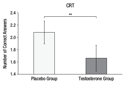
Figure 6.4: Figure 2A from Nave, Nadler, Zava, and Camerer (2017) which you should replicate
- Write code in the t4 code chunk to reproduce a version of Figure 2a - shown above. Before you create the plot, replace the
NULLto make a tibble calledcrt_meanswith the mean and standard deviation of the number ofCorrectAnswersfor each group. - Use
crt_meansas the source data for the plot.
Hint: you will need to check out recode() to get the labels of treatments right. Again this webpage is highly recommended: https://debruine.github.io/posts/recode/
Don't worry about including the error bars (unless you want to) or the line indicating significance in the plot. Do however make sure to pay attention to the labels of treatments and of the y-axis scale and label. Reposition the x-axis label to below the Figure. You can use colour if you like.
crt_means <- NULL

## TODO: add lines of code using ggplot
6.4.6 Task 5: Interpreting your Figure
Always good to do a slight recap at this point to make sure you are following the analysis. Replace the NULL in the t5 code chunk below with the number of the statement that best describes the data you have calculated and plotted thus far. Store this single value in answer_t5:
The Testosterone group (M = 2.10, SD = 1.02) would appear to have fewer correct answers on average than the Placebo group (M = 1.66, SD = 1.18) on the Cognitive Reflection Test suggesting that testosterone does in fact inhibit the ability to override incorrect intuitive judgements with the correct response.
The Testosterone group (M = 1.66, SD = 1.18) would appear to have more correct answers on average than the Placebo group (M = 2.10, SD = 1.02) on the Cognitive Reflection Test suggesting that testosterone does in fact inhibit the ability to override incorrect intuitive judgements with the correct response.
The Testosterone group (M = 1.66, SD = 1.18) would appear to have fewer correct answers on average than the Placebo group (M = 2.10, SD = 1.02) on the Cognitive Reflection Test suggesting that testosterone does in fact inhibit the ability to override incorrect intuitive judgements with the correct response.
The Testosterone group (M = 2.10, SD = 1.02) would appear to have more correct answers on average than the Placebo group (M = 1.66, SD = 1.18) on the Cognitive Reflection Test suggesting that testosterone does in fact inhibit the ability to override incorrect intuitive judgements with the correct response.
answer_t5 <- NULL6.4.7 Task 6: t-test
Now that we have calculated the descriptives in our study we need to run the inferentials. In the t6 code chunk below, replace the NULL with a line of code to run the t-test taking care to make sure that the output table has the Placebo mean under Estimate1 (group 0) and Testosterone mean under Estimate2 (group 1). Assume variance is equal and use broom::tidy() to sweep and store the results into a tibble called t_table.
t_table <- NULL6.4.8 Task 7: Reporting results
In the t7A code chunk below, replace the NULL with a line of code to pull out the df from t_table. This must be a single value stored in t_df.
t_df <- NULLIn the t7B code chunk below, replace the NULL with a line of code to pull out the t-value from t_table. Round it to three decimal places. This must be a single value stored in t_value.
t_value <- NULLIn the t7C code chunk below, replace the NULL with a line of code to pull out the p-value from t_table. Round it to three decimal places. This must be a single value stored in p_value.
p_value <- NULLIn the t7D code chunk below, replace the NULL with a line of code to calculate the absolute difference between the mean number of correct answers for the Testosterone group and the Placebo group. Round it to three decimal places. This must be a single value stored in t_diff.
t_diff <- NULLIf you have completed t7A to t7D accurately, then when knitted, one of these statements below will produce an accurate and coherent summary of the results. In the t7E code chunk below, replace the NULL with the number of the statement below that best summarises the data in this study. Store this single value in answer_t7e
- The testosterone group performed significantly better ( fewer correct answers) than the placebo group, t() = , p = .
- The testosterone group performed significantly worse ( fewer correct answers) than the placebo group, t() = , p = .
- The testosterone group performed significantly better ( more correct answers) than the placebo group, t() = , p = .
- The testosterone group performed significantly worse ( fewer correct answers) than the placebo group, t() = , p = .
answer_t7e <- NULLJob Done - Activity Complete!
Well done, you are finshed! Now you should go check your answers against the solutions at the end of this Chapter. You are looking to check that the resulting output from the answers that you have submitted are exactly the same as the output in the solution - for example, remember that a single value is not the same as a coded answer. Where there are alternative answers, it means that you could have submitted any one of the options as they should all return the same answer. If you have any questions please post them on the available forums or ask a member of staff.
On to the next chapter!
6.5 Solutions to Questions
Below you will find the solutions to the questions for the Activities for this chapter. Only look at them after giving the questions a good try and speaking to the tutor about any issues.
6.5.1 PreClass Activities
6.5.1.1 PreClass Task 1
ns_data <- tibble(participant = 1:22,
                  valid_rt = c(631.2,800.8,595.4,502.6,604.5,
                               516.9,658.0,502.0,496.7,600.3,
                               714.6,623.7,634.5,724.9,815.7,
                               456.9,703.4,647.5,657.9,613.2,
585.4,674.1))6.5.1.2 PreClass Task 2
woods_mean <- 590

n_participants <- ns_data %>%
  filter(valid_rt > woods_mean) %>%
nrow()- Giving an n_participants value of 16
6.5.1.3 PreClass Task 3
- You can use the density function:
sum(dbinom(n_participants:nrow(ns_data), nrow(ns_data), .5))## [1] 0.0262394- Or, the cumulative probability function:
pbinom(n_participants - 1L, nrow(ns_data), .5, lower.tail = FALSE)## [1] 0.0262394- Or, If you were to plug in the numbers directly into the code:
sum(dbinom(16:22,22, .5))## [1] 0.0262394- Or, finally, remembering we need to specify a value lower than our minimum participant number as
lower.tail = FALSE.
pbinom(15, 22, .5, lower.tail = FALSE)## [1] 0.0262394It is better practice to use the first two solutions, which pull the values straight from ns_data, as you run the risk of entering an error into your code if you plug in the values manually.
6.5.1.4 PreClass Task 4
- For
ns_data_meanusesummarise()to calculate the mean and thenpull()the value. - For
ns_data_sdusesummarise()to calculate the sd and thenpull()the value.
# the mean
ns_data_mean <- ns_data %>%
  summarise(m = mean(valid_rt)) %>%
  pull(m)

# the sd
ns_data_sd <- ns_data %>%
  summarise(sd = sd(valid_rt)) %>%
  pull(sd)
NOTE: You could print them out on the screen if you wanted to "\n" is the end of line symbol so that they print on different lines
cat("The mean number of hours was", ns_data_mean, "\n")
cat("The standard deviation was", ns_data_sd, "\n")
## The mean number of hours was 625.4636
## The standard deviation was 94.306936.5.1.5 PreClass Task 5
t_obs <- (ns_data_mean - woods_mean) / (ns_data_sd / sqrt(nrow(ns_data)))- Giving a t_obs value of 1.7638067
6.5.1.6 PreClass Task 6
If using values straight from ns_data, and multiplying by 2 for a two-tailed test, you would do the following:
pval <- pt(abs(t_obs), nrow(ns_data) - 1L, lower.tail = FALSE) * 2L- Giving a pval of 0.0923092
But you can also get the same answer by plugging the values in yourself - though this method runs the risk of error and you are better off using the first calculation as those values come straight from ns_data. :
pval2 <- pt(t_obs, 21, lower.tail = FALSE) * 2- Giving a pval of 0.0923092
6.5.1.7 PreClass Task 7
The t-test would be run as follows, with the output shown below:
t.test(pull(ns_data, valid_rt), mu = woods_mean)##
## One Sample t-test
##
## data: pull(ns_data, valid_rt)
## t = 1.7638, df = 21, p-value = 0.09231
## alternative hypothesis: true mean is not equal to 590
## 95 percent confidence interval:
## 583.6503 667.2770
## sample estimates:
## mean of x
## 625.46366.5.1.8 PreClass Task 8
According to the one-sample t-test these participants are responding in a similar manner as the participants from the original study, and as such, we may be inclined to assume that the recruitment process of our pilot experiment is working well.
However, according to the binomial test the participants are responding differently from the original sample. So which test result should you take as the finding?
Keep in mind that the binomial test is very rough and categorises participants into yes or no. The one-sample t-test uses much more of the available data and to some degree would give a more accurate answer. However, the fact that two tests give really different answers may give you reason to question whether or not the results are stable and potentially you should look to gather a larger sample to get a more accurate representation of the population.
6.5.2 InClass Activities
6.5.2.1 InClass Task 1
library("tidyverse")
library("broom") # you'll need broom::tidy() later

evaluators <- read_csv("evaluators.csv")

evaluators %>%
  summarize(mean_age = mean(age, na.rm = TRUE))

evaluators %>%
  count(sex)

# If using `recode()`:
evaluators %>%
  count(sex) %>%
mutate(sex_names = recode(sex, "1" = "male", "2" = "female"))- The mean age of the evaluators was 30.9
- The standard deviatoin of the age of the evaluators was 6.24
- There were 4 males and
e_count %>% filter(sex_names == "female") %>% pull(n)females, with 5 people not stating a sex.
6.5.2.2 InClass Task 2
- load in the data
ratings <- read_csv("ratings.csv")- First pull out the ratings associated with intellect
iratings <- ratings %>%
filter(Category %in% c("competent", "thoughtful", "intelligent"))- Next calculate means for each evaluator
imeans <- iratings %>%
  group_by(eval_id) %>%
summarise(Rating = mean(Rating))- Mutate on the Category variable. This way we can combine with 'impression' and 'hire' into a single table which will be very useful!
imeans2 <- imeans %>%
  mutate(Category = "intellect")
And then combine all the information in to one single tibble.
ratings2 <- ratings %>%
  filter(Category %in% c("impression", "hire")) %>%
  bind_rows(imeans2) %>%
  inner_join(evaluators, "eval_id") %>%
  select(-age, -sex) %>%
arrange(eval_id, Category)6.5.2.3 InClass Task 4
- First we calculate the group means:
group_means <- ratings2 %>%
  group_by(condition, Category) %>%
  summarise(m = mean(Rating), sd = sd(Rating))
## `summarise()` has grouped output by 'condition'. You can override using the `.groups` argument.- And we can call them and look at them by typing:
group_means- Now to just look at intellect ratings we need to filter them into a new tibble:
intellect <- filter(ratings2, Category == "intellect")- And then we run the actual t-test and tidy it into a table.
t.test()requires two vectors as inputpull()will pull out a single column from a tibble, e.g. Rating from intellecttidy()takes information from a test and turns it into a table. Try running the t.test with and without piping intotidy()to see what it does differently.
intellect_t <- t.test(intellect %>% filter(condition == "listened") %>% pull(Rating),
                      intellect %>% filter(condition == "read") %>% pull(Rating),
                      var.equal = TRUE) %>%
tidy()- Now we repeat for HIRE and IMPRESSION
hire <- filter(ratings2, Category == "hire")
hire_t <- t.test(hire %>% filter(condition == "listened") %>% pull(Rating),
                      hire %>% filter(condition == "read") %>% pull(Rating),
                 var.equal = TRUE) %>%
tidy()- And for Impression
impress <- filter(ratings2, Category == "impression")
impress_t <- t.test(impress %>% filter(condition == "listened") %>% pull(Rating),
                    impress %>% filter(condition == "read") %>% pull(Rating),
                    var.equal = TRUE) %>%
tidy()- Before combining all into one table showing all three t-tests
results <- bind_rows("hire" = hire_t,
                     "impression" = impress_t,
                     "intellect" = intellect_t, .id = "id")

results6.5.2.4 Going Further with your coding
An alternative solution to Task 4: There is actually a quicker way to do this analysis of three t-tests which you can have a look at below if you have the time. This uses very advanced coding with some functions we won't really cover in this book. Do not worry if you can't quite follow it though; the main thing is to understand what we covered in the main chapter activities - the outcome is the same.
ratings2 %>%
  group_by(Category) %>%
  nest() %>%
  mutate(ttest = map(data, function(x) {
    t.test(Rating ~ condition, x, var.equal = TRUE) %>%
      tidy()
  })) %>%
  select(Category, ttest) %>%
unnest(cols = c(ttest))| Category | estimate | estimate1 | estimate2 | statistic | p.value | parameter | conf.low | conf.high | method | alternative |
|---|---|---|---|---|---|---|---|---|---|---|
| hire | 1.825397 | 4.714286 | 2.888889 | 2.620100 | 0.0126745 | 37 | 0.4137694 | 3.237024 | Two Sample t-test | two.sided |
| impression | 1.894180 | 5.968254 | 4.074074 | 2.850766 | 0.0070911 | 37 | 0.5478846 | 3.240475 | Two Sample t-test | two.sided |
| intellect | 1.986773 | 5.634921 | 3.648148 | 3.525933 | 0.0011444 | 37 | 0.8450652 | 3.128480 | Two Sample t-test | two.sided |
6.5.3 Test Yourself Activities
6.5.3.2 Assignment Task 1B: Loading in the data
- Use
read_csv()to read in data!
crt <- read_csv("data/06-s01/homework/CRT_Data.csv")crt <- read_csv("CRT_Data.csv")6.5.3.3 Assignment Task 2: Selecting only relevant columns
The key columns are:
- ID
- Treatment
- CorrectAnswers
Creating crt2 which is a tibble with 3 columns and 243 rows.
crt2 <- select(crt, ID, Treatment, CorrectAnswers)6.5.3.4 Assignment Task 3: Verify the number of subjects in each group
The Participants section of the article contains the following statement:
243 men (mostly college students; for demographic details, see Table S1 in the Supplemental Material available online) were randomly administered a topical gel containing either testosterone (n = 125) or placebo (n = 118).
In the t3 code block below, replace the NULLs with lines of code to calculate:
The number of men in each Treatment. This should be a tibble/table called
cond_countscontaining a column calledTreatmentshowing the two groups and a column callednwhich shows the number of men in each group.The total number of men in the sample. This should be a single value, not a tibble/table, and should be stored in
n_men.
You know the answer to both of these tasks already. Make sure that your code gives the correct answer!
For cond_counts, you could do:
cond_counts <- crt2 %>% group_by(Treatment) %>% summarise(n = n())Or alternatively
cond_counts <- crt2 %>% count(Treatment)For n_men, you could do:
n_men <- crt2 %>% summarise(n = n()) %>% pull(n)Or alternatively
n_men <- nrow(crt2)Solution:
When formatted with inline R code as below:
`r n_men` men (mostly college students; for demographic details, see Table S1 in the Supplemental Material available online) were randomly administered a topical gel containing either testosterone (n = `r cond_counts %>% filter(Treatment == 1) %>% pull(n)`) or placebo (n = `r cond_counts %>% filter(Treatment == 0) %>% pull(n)`).
should give:
243 men (mostly college students; for demographic details, see Table S1 in the Supplemental Material available online) were randomly administered a topical gel containing either testosterone (n = 125) or placebo (n = 118).
6.5.3.5 Assignment Task 4: Reproduce Figure 2A
You could produce a good representation of Figure 2A with the following approach:
crt_means <- crt2 %>%
  group_by(Treatment) %>%
  summarise(m = mean(CorrectAnswers), sd = sd(CorrectAnswers)) %>%
  mutate(Treatment = recode(Treatment, "0" = "Placebo", "1" = "Testosterone Group"))

ggplot(crt_means, aes(Treatment, m, fill = Treatment)) +
  geom_col() +
  theme_classic() +
  labs(x = "CRT", y = "Number of Correct Answers") +
  guides(fill = "none") +
  scale_fill_manual(values = c("#EEEEEE","#AAAAAA")) +
  coord_cartesian(ylim = c(1.4,2.4), expand = TRUE)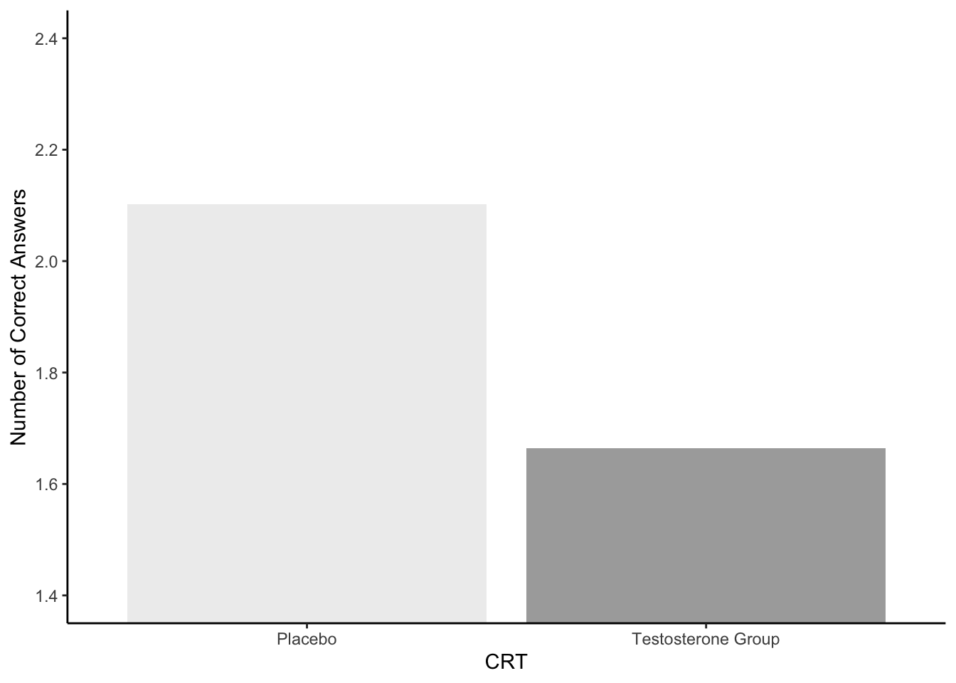
Figure 6.5: A representation of Figure 2A
6.5.3.6 Assignment Task 5: Interpreting your Figure
Option 3 is the correct answer given that:
The Testosterone group (M = 1.66, SD = 1.18) would appear to have fewer correct answers on average than the Placebo group (M = 2.10, SD = 1.02) on the Cognitive Reflection Test suggesting that testosterone does in fact inhibit the ability to override incorrect intuitive judgements with the correct response.
answer_t5 <- 36.5.3.7 Assignment Task 6: t-test
You need to pay attention to the order when using this first approach, making sure that the 0 group are entered first. This will put the Placebo groups as Estimate1 in the output. In reality it does not change the values, but the key thing is that if you were to pass this code on to someone, and they expect Placebo to be Estimate1, then you need to make sure you coded it that way.
t_table <- t.test(crt2 %>% filter(Treatment == 0) %>% pull(CorrectAnswers),
                  crt2 %>% filter(Treatment == 1) %>% pull(CorrectAnswers),
                  var.equal = TRUE) %>%
tidy()- Alternatively, you could use what is known as the formula approach as shown below. Here you state the
DV ~ IVand you say the name of the tibble indata = .... You just need to make sure that the columns you state as the DV and the IV are actually in the tibble!
t_table <- t.test(CorrectAnswers ~ Treatment, data = crt2, var.equal = TRUE) %>% tidy()6.5.3.8 Assignment Task 7: Reporting results
- The degrees of freedom (df) is found under
parameter
t_df <- t_table$parameter- An alternative option for this would be as follows, using the
pull()method. This would work for B to D as well
t_df <- t_table %>% pull(parameter)- The t-value is found under
statistic
t_value <- t_table$statistic %>% round(3)- The p-value is found under
p.value
p_value <- t_table$p.value %>% round(3)- The absolute difference between the two means can be calculated as follows:
t_diff <- (t_table$estimate1 - t_table$estimate2) %>% round(3) %>% abs()If you have completed t7A to t7D accurately, then when knitted, Option 4 would be stated as such
The testosterone group performed significantly worse (0.438 fewer correct answers) than the placebo group, t(241) = 3.074, p = 0.002
and would therefore be the correct answer!
answer_t7e <- 4Chapter Complete!
6.6 Additional Material
Below is some additional material that might help you understand the tests in this Chapter a bit more as well as some additional ideas.
More on t.test() - vectors vs. formula
A quick note on running the t-test in two different ways. In the lab we showed you how to run a t-test on a between-subjects design. This is the Welch's t-test version of the code from the lab:
t_table <- t.test(crt2 %>% filter(Treatment == 0) %>% pull(CorrectAnswers),
                  crt2 %>% filter(Treatment == 1) %>% pull(CorrectAnswers),
                  var.equal = FALSE) %>%
  tidy()
This is sometimes referred to as the vector approach, and what the code is doing is taking each groups' data as a vector input. For example, if you were to just look at the data for the Treatment 0 group then that line of code:
crt2 %>% filter(Treatment == 0) %>% pull(CorrectAnswers)shows just these values:
##   [1] 2 2 3 3 3 2 1 0 2 0 2 1 3 2 2 3 1 3 2 3 2 0 2 3 3 3 3 2 2 2 3 0 3 3 3 0 0
##  [38] 3 3 1 3 1 2 3 3 1 3 3 3 3 2 3 2 2 2 2 3 3 1 3 1 0 3 1 3 1 2 3 3 0 2 2 2 3
##  [75] 1 2 3 0 3 1 1 3 3 0 1 0 3 2 2 3 1 3 3 2 3 1 3 2 3 3 3 3 3 3 2 3 3 2 2 0 3
## [112] 0 1 2 2 3 3 3
And likewise the Treatment 1 line of code just gives these values:
##   [1] 2 0 0 1 3 0 0 2 2 3 1 3 3 1 0 2 1 0 0 3 2 0 3 0 3 3 3 0 2 0 3 3 3 1 0 0 1
##  [38] 2 3 2 2 2 3 3 1 0 3 0 1 1 1 0 0 1 2 3 3 0 2 2 3 3 2 3 3 3 3 3 3 1 2 3 1 1
##  [75] 2 3 3 0 2 2 1 1 2 3 0 0 3 0 1 2 0 0 0 0 3 1 3 2 2 2 1 2 3 3 0 3 1 0 1 2 0
## [112] 2 2 2 3 2 3 3 3 0 3 0 1 2 3
And the t.test() function is just saying this is group 1's data, this is group 2's data, and I am comparing them. However the eagle-eyed of you will have seen in the solution an alternative code, that looks like:
t_table <- t.test(CorrectAnswers ~ Treatment, data = crt2, var.equal = FALSE) %>% tidy()This is the formula method and if you look at the structure of crt2 (the first 6 rows are shown below) you get an idea of how the formula approach works:
| ID | Treatment | CorrectAnswers |
|---|---|---|
| 11 | 1 | 2 |
| 12 | 1 | 0 |
| 13 | 1 | 0 |
| 14 | 1 | 1 |
| 15 | 1 | 3 |
| 16 | 1 | 0 |
The formula approach works as t.test(DV ~ IV, data = my_data) where:
- DV is the name of the column with your responses (e.g. mean reaction time)
- IV is the name of the column with your groups (in categorical form - e.g. 1 vs 0)
~means "by" or "based on" or "split up by". So test the DV based on the IV grouping- and my_data is the name of your tibble.
Whichever approach you use, the observed t-value, p-value, and df (parameter) should be the same! What might change is what the t-test considers as group 1 and what it considers group 2. And from your knowledge of the t-test formula, this will affect whether your t-test is positive or negative. For example:
t_table <- t.test(crt2 %>% filter(Treatment == 0) %>% pull(CorrectAnswers),
                  crt2 %>% filter(Treatment == 1) %>% pull(CorrectAnswers),
                  var.equal = FALSE) %>%
  tidy()
Gives the t-value of t = 3.09, whereas if you switch the order of inputting the Treatment groups as such:
t_table <- t.test(crt2 %>% filter(Treatment == 1) %>% pull(CorrectAnswers),
                  crt2 %>% filter(Treatment == 0) %>% pull(CorrectAnswers),
                  var.equal = FALSE) %>%
  tidy()
You get a t-value of t = -3.09. Same value (or magnitude) just one is positive and the other is negative, because the order of who is Group 1 and who is group 2 is switched. And just for comparion, the formula approach:
t_table <- t.test(CorrectAnswers ~ Treatment, data = crt2, var.equal = FALSE) %>% tidy()Gives a t-value of t = 3.09. So again the same magnitude but you are not controlling who is Group 1 and who is Group 2.
Long story short is that both methods, if used appropriately, run the same analysis. The benefit of the vector approach is that you can dictate in your analysis who is Group 1 and who is Group 2. And that is really the only difference.
Misleading and Appropriate Barplots
Misleading Barplots
The data used in the PreClass activities allows us to show you something that you might find interesting. As we mentioned back in Chapter 3 on visualisation, the barplot is becoming less frequently used, as summarised in this blog: One simple step to improve statistical inferences. The data we have used today demonstrate the point that a simple barplot can actually be somewhat misleading about the data. Have a look at the figure below. Both bars represent the data from our 22 Normal Sleep participants. The column on the left, hide_data, is a standard representation (albeit without error bars) whereas the column on the right, show_data, demonstrates the issue. Looking at the column on the left, the assumption is that all the data is around the peak of the column. However, looking at the column on the right, we can see that this is not the case and there are participants both above and below the mean by approximately 100 ms. This misleading perception, when the data is hidden, was tested and shown to exist in participants viewing these figures by Newman and Scholl (2012) which you can read up on if you like.
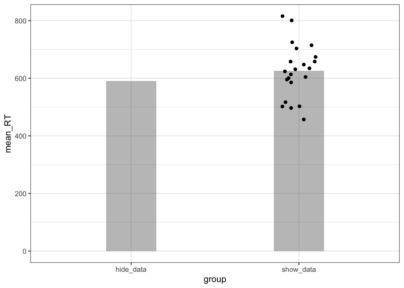
Figure 6.6: How representative are barplots of the actual spread of the data!
The function we use to show the data points is geom_jitter() and it gets added to a visualisation pipeline just like other geom_?()s that we have used; your code will look like something like this:
ggplot(my_data, aes(x = my_x_variable, y = my_y_variable)) +
  geom_col() +
  geom_jitter(width = .1)
Look out for it in the coming chapters but the main thing to keep in mind is that barplots can be misleading and displaying the individual data may be more informative - particularly when the response measured creates a spread of data.
Appropriate Barplots
That said, barplots do have their place in data analysis and research methods. The best time to use a barplot is when the value is a count - i.e. when the value had no variability in it. A great example of this is in observational research using categorical data. Think about the table we simulated for the chi-squre data as part of the Additional Materials in Chapter 5. Here is that table again:
| Groups | No | Unsure | Yes | Total |
|---|---|---|---|---|
| A | 17 | 18 | 15 | 50 |
| B | 18 | 14 | 18 | 50 |
We have two groups with three possible responses and each participants can only give one response. What that means, for example, is that there is no variation in the number of people who in Group A said No - it is exactly 17 people. Likewise, exactly 14 people in Group B said unsure. So here a barplot actually makes sense to use as it accurately reflects the value in that group/condition and no data is hidden. The plot for the above table might look like this:
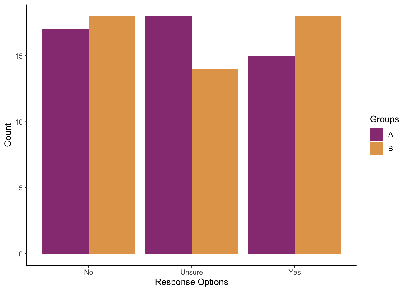
Figure 6.7: A barplot works well with categorical data
In short, the main message about any visualisation is about accurately and clearly conveying that information to your reader. If there is a spread of data within a variable then try to show that more clearly with error bars and data points, perhaps even using a violin plot instead of a barplot. If however there is no spread of data within a variable then a barplot works well.
Analysing chi-squares
Finally, to round of this additional material, we thought it might be handy to show how to run a chi-square analysis. We cover the chi-square more in lectures but adding it here might help some people. We won't really look at the hand calculations, but you will know that the formula for the chi-square is:
\(x_c^2 = \sum\frac{(O_i - E_i)^2}{E_i}\)
- where \(x_c^2\) is the chi-square symbol - often simplified to \(x_2\)
- \(O_i\) is the observed value of group {i} and
- \(E_i\) is the expected value of group {i}
And we can use the data from above to show how to quickly run the chi-square analysis on the table. First we need to tidy up the table to get rid of the Groups and Total columns, leaving us with a tibble called chi_table that has this structure:
| No | Unsure | Yes |
|---|---|---|
| 17 | 18 | 15 |
| 18 | 14 | 18 |
Now to analyse the data we use the chisq.test() function. There are really only two arguments you need to think about:
- your data - for us stored in
chi_table - and whether to set
correctas TRUE or FALSE. This is Yates' Continuity Correction. The default is set as TRUE but a lot of people set it as FALSE so we will select that today.
And we run the analysis as such:
chisq_result <- chisq.test(chi_table, correct = FALSE) %>% tidy()Giving the following result:
| statistic | p.value | parameter | method |
|---|---|---|---|
| 0.8012987 | 0.6698849 | 2 | Pearson's Chi-squared test |
And could be written up as \(x_c^2\)(df = 2, N = 100) = 0.8, p = 0.67. And if you wanted to check the output and calculate the data by hand, or needed to do further analysis, you can see the expected values by doing the analysis but not tidying it, as follows:
chisq_untidy <- chisq.test(chi_table, correct = FALSE)

chisq_untidy$expected
## No Unsure Yes
## [1,] 17.5 16 16.5
## [2,] 17.5 16 16.5And if you wanted the expected values for just one of the groups - say the second group, Group B:
chisq_untidy$expected[2,]## No Unsure Yes
## 17.5 16.0 16.5Or even just the observed values to check you entered the data correctly:
chisq_untidy$observed## No Unsure Yes
## [1,] 17 18 15
## [2,] 18 14 18We will leave that there but hopefully this gives you some additional insight into how to analyse a chi-square test.
End of Additional Material!