Lab 1 Starting with R Markdown

1.1 Overview

A key goal of any researcher is to carry out an experiment and to tell others about it. One of the main ways we as Psychologists do this is through publication of a journal article. There are numerous ways that people combine different software to create a journal article, but a more recent innovation in the field that we want you to know about is creating reports and articles through R Markdown. If you like, you can see an example from a research team in our school in this recent PLOS article. A link within the article methods section (this one - https://osf.io/eb9dq/) allows you to see the one file that creates the whole manuscript. Obviously you won't be writing full journal articles just yet but you will use R Markdown throughout this lab series to do assignments. You could also use it in other subjects to write reports, or to make yourself a portfolio of hints, tips, and study aids as we suggest throughout the labs.

Today, we will start by showing you some of skills in using R Markdown efficiently.

In this lab you will learn:

What is R Markdown?
How to create an R Markdown file and knit it.
How to add code and edit rules in your R Markdown file.
How to format your text.

1.1.1 What is R Markdown?

R Markdown (abbreviated as Rmd) is a great way to create dynamic documents through embedded chunks of code. These documents are self-contained and fully reproducible which makes it very easy to share. For more information about R Markdown feel free to have a look at their main webpage sometime: The R Markdown Webpage. The key advantage of R Markdown is that it allows you to write code into a document, along with regular text, and then knit it using the package knitr() to create your document as either a webpage (HTML), a PDF, or Word document (.docx).

Throughout the labs you will see little tabs that give more information, answers to quick questions, helpful hints, solutions to tasks, or suggestions for information you want to note down somewhere. You do not have to read them all and you will find they get less as the course progresses, but they might help you if you are stuck on something.

Knit is what we say when we want to turn our R Markdown file into either a webpage, PDF, or a Word document. Often in the labs you will hear someone say, "Have you tried knitting it?" or "What happens when you knit it?". This simply means what happens when you try turning your file into a pdf or webpage.

For any of the practical data assignments, one check to run before submitting is to knit your code to an html (webpage) file and then see if you can open that file in your browser. This doesn't check that your code is correct. It does however confirm that your code runs and has no critical issues in it that would stop your code from running. A very valuable check.

1.1.2 Advantages of using R Markdown

The output is one file that includes figures, text and citations. No additional files are needed so it's easy to keep all your work in one place.
R code can be put directly into an R Markdown report so it is not necessary to keep your writing (e.g. a Word document) and your analysis (e.g. your R script) separate.
Including the R code directly lets others see how you did your analysis - this is a good thing for science! It is both reproducible and transparent, key components of Open Science!
You write your report in plain text, a non software-specific format that is easy to share, so it's not necessary to learn any new coding such as HTM, but can create various outputs depending on what you need.

1.1.3 Creating an R Markdown (.Rmd) File

In this lab you're going to create your own R Markdown document. Knowing how to do this will:

help you navigate R Markdown, in turn with submitting homework assignments, and
help you to create your own reports using it.

If at any point you are unsure about how to do something remember to think about where you can get help. There is an R Markdown Cheatsheet on the top menu under Help >> Cheatsheets or do what we do, google it. For example, if I forget how to put words in bold, I could simply go to Google and type "rmarkdown bold" and no doubt get a lot of useful hints. There is nothing wrong with this. Nobody is expecting you to keep every function in your head; we all need reminders. You will find some elements stick in your head better than others. So remember, google is your friend!

Quickfire Questions

We have put questions throughout to help you test your knowledge. When you type in or choose the correct answer, the dashed box will change color and become solid.

From the following options, why are we creating an R Markdown document instead of simply using an R script?

So there's more than one answer to this question! R Markdown can combine report writing and analysis, providing open access for others to examine data, and create more Reproducible Science. But what about the incorrect answer? R Scripts do in fact run R code as you may remember from Level 1 labs. The key difference is that R Scripts cannot really be used for documentation and creating reports as easily - this is where R Markdown is used to ensure your code can be added to all the other information of your research and can be reproduced by others.

1.1.4 One last thing before beginning!

Before working through the rest of this Lab you may want to watch the short videos on the Moodle pages and the Level 1 PsyTeachR Grassroots book reminding you about the skills we want you have already learnt through using R and RStudio, and the various file formats you will be working with.

1.2 PreClass Activiy

Having read the Overview for this lab, and the reason behind using R, we are now going work on making a reproducible code. If you have a laptop, it is best to install R and Rstudio on that for you to use. The videos on Moodle and in the Grassroots book gives a reminder of how to install R and Rstudio. If you don't have it installed yet you can just read along today and try it out when you have access to a machine in the labs or online through a cloud, server or remote access.

1.2.1 Let's Begin

Create a new R Markdown file (.Rmd) by opening Rstudio, and then on the top menu, selecting File >> New File >> R Markdown.... You should now see the following dialog box:

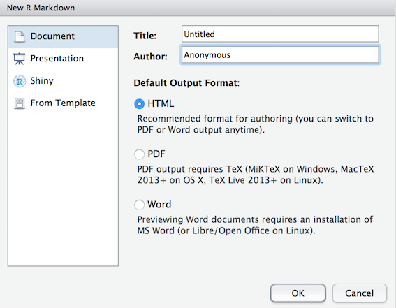
Figure 1.1: Starting an R Markdown file

Click Document on the left-hand panel and then give your document a Title.

This is your file so call it what you want but make sure it is informative to you and your reader.

Put your name or your student ID in the Author field as you are the author. For now we will focus on making an HTML output, so make sure that is selected as shown in Figure 1.1 then hit OK when you have done so. You should now have an .Rmd file open in Rstudio.

The first thing you will see in your R Markdown file is a header section enclosed at the top and bottom by ---. Technically called the yaml header, this section lists the title, author, date and output format. The layout of the header is very precise and will look like that shown in Figure 1.2, which is currently set to output as HTML.

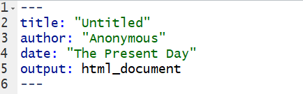
Figure 1.2: An Rmd yaml header

By default the file header includes the info shown in Figure 1.2 but there are many other options available. You can learn more about this in your spare time if you like through these links: http://rmarkdown.rstudio.com/html_document_format.html for .html options or http://rmarkdown.rstudio.com/pdf_document_format.html for .pdf options.

BUT WAIT!! What if you spelt your name wrong? How would you change this?

The long way would be to close the file and start again. The shorter way would be to just correct the info in the header - just remember to keep between the quotes. E.g. "Si Cologe" instead of "Untitled"

1.2.2 Code Chunks

Immediately below the header information you will see the default setup code chunk as shown in Figure 1.3. Most of the time, in this lab series, you will not edit the information in this chunk. Instead, you will add information, text, code, and chunks, below this chunk.

Figure 1.3: The defualt setup code chunk

In RMarkdown you can type any text you want directly in the document just as you would in a word document. However, if you want to include code you need to include it in one of these code chunks similar to Figure 1.3. Code chunks start with a line that contains three backwards apostrophes ` (these are called grave accents - often in the top-left of QWERTY keyboards), and then a set of curly brackets with the letter r inside:

```{r}```

You will always need both of these parts to create a code chunk:

The three back ticks ` are the part of the Rmd file that says this is code being inserted into my document.
The {r} part says that you are specifically including R code.

The default setup code chunk provides some basic options for your R Markdown file for when it knits your work. As above, for now, it is best to leave this particular code chunk alone. Instead we will show you how to use R Markdown by editing the code chunks that come after this default chunk.

The next code chunk in your file will look a bit like this:

```{r cars}

summary(cars)

```

Within the curly brackets, on the first line of the chunk, the word cars is included after the letter r. This is simply the name or the label for the code chunk and it really could have been called anything. For example, you could have called this code chunk cars1 and a later chunk cars2 to show it was the first and second chunk relating to cars. Whilst it is always advisable you name your code chunks, you do not need to name them. However, if you do put in names for the chunks do not use the same name twice as this will cause your script to crash when you knit it, e.g. Do not use data and data; instead maybe use personality_data and participant_info or whatever makes sense to what you are doing in the chunk. OK? Different names for different chunks! They are all individual.

Remember knitting just means converting or rendering your file as a pdf, webpage, etc. Crashing means that you had an error in your code that stopped your knitting from working or finishing. You can usually find the problem line of code from the error message you'll see.

The second line in the above code chunk is the R code we have written: summary(cars). In this case, we are just asking for a summary() of the inbuilt dataset cars. R has a lot of inbuilt datasets for you to practice on; cars is one of these.

The third line closes off the code chunk, again with the three backwards apostrophes. This means that whatever is contained between the first and third lines will be the code that is run.

When people are first starting out using R Markdown, a common issue is code not working because they have started the code chunk correctly, but have forgotten to close it at the bottom with the three backticks. Remember, three backticks to open, three backticks to close, and in our chunk we bind them.

Quickfire Questions

From the following options what was the name, or label, of the default setup code chunk (i.e. the first code chunk in an R Markdown file)?

If you look at the default setup code chunk you can see the code chunk has the name setup. include=FALSE is a rule which we will explain in a little bit.

1.2.3 Knitting Code

Now would be a good time to try knitting your file to see what the code chunks do. You can do this using the Knit button at the top of the RStudio screen:

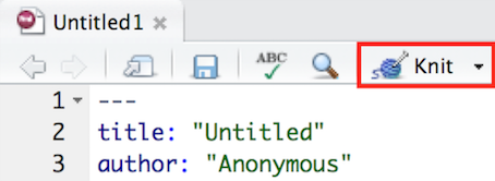
Figure 1.4: The knit button. Clicking this will knit your file.

When you click Knit it will ask you to save the file as an .Rmd file. Call the file L2Psych_Lab1_Preclass.Rmd and save it in a folder where you will keep all the information for this lab. When working in the Psychology labs or the University Library you need to save in a location or drive space that you have full access to and can save files to. The best one on campus is your M: drive. If using your own device then anywhere you can save the file should work. However, having a good folder structure will help you navigate the labs better.

It would be very beneficial to create a folder in your M: drive that will contain all your practical lab work for the rest of Level 2. Maybe something like Psychology_Level_2_Lab_Work and then have folders within that for each lab, e.g Lab1. The clearer the structure of these folders the easier it will be to find and use your files again! This is important as one thing we will keep telling you to do is LOOK BACK (politely) at what you previously did.

A good way to think about this is if you have an exam, it isn't helpful to be told the location of your exam is 'Glasgow Uni' (i.e. a large folder of many locations). Instead you would need to be told the specific building (a folder within your larger folder), but more specifically the room number in the building where your exam is taking place (the folder which you are working from).

Couple of tips:

Avoid spaces in file names and folder names. It can make life really complicated and is a bad habit to start with. Use underscores between words in filenames and folder names.
Never call your folder "R". This will crash your R and potentially lead you to having to reinstall both R and Rstudio. When Rstudio opens it looks for a folder called R which it expects to contain the software and libraries. If they aren't there because it is now looking in a different folder with the same name, things go wrong. Sort of like the Sally-Anne False Belief task, but not as exciting.

After saving the file, a webpage should appear. The first thing to notice is that some lines in the code chunks have disappeared: the ```{r} and the closing ``` in your code chunk have gone. Whenever you knit an R Markdown file these lines will disappear leaving only the code within. You'll also notice that the output of the code is also now showing in your webpage. In the next section we will show you how to control showing the output of your code, or not, through adding rules.

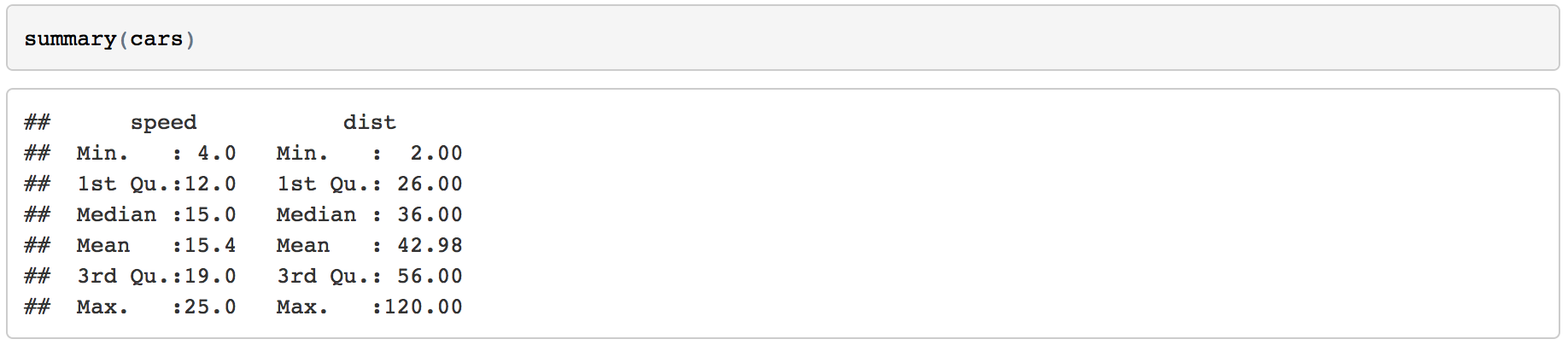
Figure 1.5: The knitted summary output

1.2.4 Adding Code Chunk Rules and Options

It can often be a good idea or even necessary to show the data or the outcome of a test in your report, for example if you were writing a report and wanted to include a table of results. But what if your code displayed a table that was 10,000 lines long? In that case we might want to not show the output and only show the code. You can do this by including a rule within the first line of your code chunk - your ```{r name, rule = option} line. You have already seen a rule before in the standard default chunk, the include rule, but there are a number of others. Let's look at some now:

First, let's look at how to hide the output but show the code. Here, we use the results = "hide" rule:

Figure 1.6: The results Rule

Add this rule into your example code chunk, as shown above, and knit the file again. What happens? Note that there is a comma separating the name of the chunk and the rule. You should now see the code only and not the data. A key thing to note here is that your code is still "running", it just isn't showing an output. For example, say your code said x <- 2 + 2. With the results = "hide" rule, you would still be running that line of code, x being assigned as 4, but you just don't see the output.

Alternatively, we can hide the code, but show the ouput by using the echo = FALSE rule:

Figure 1.7: The echo Rule

In your template Rmd file, the rule echo is set to FALSE meaning to show the figure and not the code. Change the rule in your code to echo and set it as TRUE, then knit the file again. What happens?

Remember from Level 1 where we called in libraries to our environment. The "echo = FALSE" option is useful for commands like library() when you are just calling a package into the library but don't necessarily want to display that in your final report or in your final HTML file. Another example might be if you wanted to make a plot but didn't want to include the code, you just want to show the plot in your report.

Next, say you want to hide both the code AND the output but still run the code. You can do this using the include rule:

Figure 1.8: The include Rule

Change the rule to your example code chunk, as shown above, to include = FALSE and then knit the file again. What happens? Note that here the code still runs. It just does not show you anything.

Finally, you can use the eval rule which specifies whether or not you want the code chunk you have written to be evaluated when you knit the RMarkdown file. Evaluated means to run or carry out the code. Here, the eval = FALSE rule will stop the code from being evaluated. The code will be shown because there is no rule stopping it but there will be no output because it won't get evaluated because of the eval rule being FALSE.

Figure 1.9: The eval Rule

This might be useful in cases where you want to show the code relating to how you programmed your stimuli for an experiment, but you don't necessarily want it to run as part of the R Markdown file.

We could probably do with a wee summary here:

Table 1.1: Rules! Rules! Rules!
Code	Does Code Run	Does Code Show	Do Results Show
eval = FALSE	NO	YES	NO
echo = TRUE	YES	YES	YES
echo = FALSE	YES	NO	YES
results = "hide"	YES	YES	NO
include = FALSE	YES	NO	NO

You can also mix and match rules to get the code/output to display as you want. It takes a little getting used to at first but if in doubt, just ask.

You can use RStudio's autocomplete (the tab button) to see the different options for the different rules. For example, type include = and then hit the tab button on your keyboard. You should see the options of TRUE or FALSE.

Autocomplete also works for a lot of functions you can't quite remember how to spell as well. gg-what? gg-{tab button}... Ah yes, ggplot().

Quickfire Questions

You've got a large dataset of thousands of participants' personality and happiness scores that you want to analyse and present in RMarkdown.

You want to show the code you are running in your analysis but not show the output as this would be too much to display. Note that you want the code to run. Type in the box (e.g. rule = set) how you would set the results rule to do this?
You create a plot of happiness versus neuroticism scores but you want to hide the code and only show the output. How can you do this?

The first answer should be results = "hide" as you want to show the code and run the code but not necessarily show the output of the code.

In the second question, include = FALSE technically would hide the code, but this also hides the output! echo = FALSE allows you to still see your plot while hiding the code you want hidden. code = HIDE - if only it were that simple!

Remember, the aim of these questions aren't to help you memorise these codes (no one can do that!); they're to help you gain a better understanding of how to apply these codes when you come across them in the future.

True or False, writing echo = TRUE has the same effect on the output of a code chunk as if you had no echo rule at all:

All of the code chunk rules have a default option. For example, echo, include, and eval are usually by default set to TRUE. As a result, if you don't set any echo rule, i.e. you don't specifically set echo = FALSE in your code chunk, then it is the same as setting echo = TRUE. So not specifying an option will give you the default setting for that option.

True or False, there is no difference between setting results = "hide" and eval = FALSE as they both hide the output:

With setting results = "hide", the code is evaluated and results are produced but the output is hidden. With setting eval = FALSE, the code is not evaluated and therefore no results or output have been produced. If you need your output for a later part of the code then you would might use results = "hide". If you don't need the output and just want to show the code as an example then you might use eval = FALSE.

1.2.5 Adding Inline Code

An alternative way to add code to a report is through what is called using inline code. With inline code you don't use a code chunk. Instead the code appears inline with the text. Inline code can be inserted using a back-tick, then the letter r, followed by a space, then the code you want to include, then finally another back-tick. For example, writing `r 2 + 2` would return the answer 4 when you knit the file instead of showing the code. Remember, you do not do this inside a code chunk, you do this in line with your text, e.g.:

"We ran `r 2+2` people".

Which when knitted becomes:

"We ran 4 people".

So inline coding is really useful if you want to do calculations within your text or insert values into text, say from a dataframe, to make an informative sentence. We will look at more complex examples later in the labs but again this is a really useful tool for writing manuscripts through R Markdown the more comfortable you get with it.

Quickfire Questions

You need back tick(s) to insert code chunks
Why is this inline code, `{r} 6 * 8` , not going to show the calculated answer when you knit the file? Try editing the code line in Rmarkdown and knitting it to get it to work.

All code chunks start and end with three back-ticks.
Inline coding does not use the curly brackets around the r.
All you need for inline coding is a back-tick, r, space, code, and a final back-tick.

1.2.6 Formatting the R Markdown File

The last thing we want to show you in this preclass activity is how to format your text.

When you're not writing in code chunks you can format your document in lots of different ways just like you would in a Word document (or other expensive license-based software). The R Markdown cheatsheet provides lots of information about how to do this but we will show you a couple of things that you might want to try out.

We can make text bold by including two ** (two asterisks) at the start and end of the text we want to present in bold font. For example:

"We ran **4 people**.

Which when knitted becomes:

"We ran 4 people".

Now write some text in your Rmd file and put it in bold. Knit the file to check it worked.

You could also try using italics by putting a single * (asterisk) at the start and end of the word or sentence. Try this now. Here is an example to help.

"We ran *4 people*.

Which when knitted becomes:

"We ran 4 people".

Note: italics can be difficult to read for many people and as such we have tried to avoid using it in this book. If you find some italics, where it is not necessary, please let us know and claim your reward of a packet of minstrels. Yes, a whole packet!

Finally, you might want to add headings and sub-headings to your file. For example, maybe you are writing a Psychology journal article and want to put in a header for the Introduction, Methods, Results, or Discussion sections. We do this using the # (hashtag) symbol as shown in Figure 1.10.

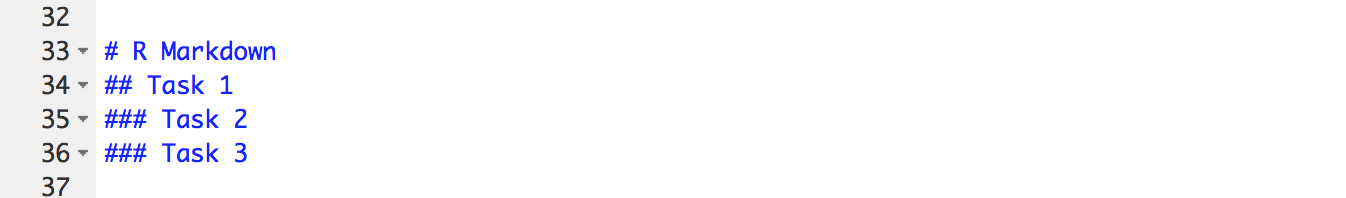
Figure 1.10: Inputting different Header levels using #s

Now, type the four main sections found in a Psychology journal article in your R Markdown file, typing each one in a separate line. These are mentioned above. Knit the file. What do these look like?

Now add a different number of #'s before each heading, with a space between the heading and the hashtag (e.g. # Introduction) and knit the file again. What do you notice about the different number of hashtags?

Quickfire Questions

If * puts words into italics, and ** puts words into bold, type in the box what might you put before (and technically after) a word to put it into italics with bold?
True or False: The more '#'s you include, the smaller the header is:
From the options, the most common order of headings found in a Psychology Journal are:

If * at the start and end of the word puts it in italics (e.g. italics) and ** puts it in bold (e.g. bold), then putting three *** at the start and end will put it in italics with bold (e.g. italics-bold).

It is true that the more #'s you use, the smaller the heading is. Word and other document writers use different headings as well. Here, # gives the biggest heading, and it gets smaller and smaller with every extra #.

Finally, in Psychology, the vast majority of journal articles are written in the format of: Introduction, Methods, Results, Discussion. This format does not always hold as some journals ask authors to use a different format, depending how much emphasis that journal (erroneously) likes to put on results over hypothesis and methods. We however teach the order stated above. The question and approach is always as important, if not more so, than the results! Which of course you know from learning about Registered Reports in the labs and lectures.

Job Done - Activity Complete!

Well done on working your way through this activity. Be sure to make notes for yourself, and to post any questions on the forums that you may have. See you in the lab!

1.3 InClass Activiy

For all the inclass activities, you will need to have completed the PreClass Activities. You may also need some cheatsheets such as The R Markdown Cheatsheet. Everything you need to complete this inclass activity can be found in those documents. We will tell you which additional material might help where we think it is appropriate.

1.3.1 R Markdown and The Experimental Design Portfolio

In the preclass activity, we asked you to start playing about with R Markdown. Now, in the lab, we are going to continue learning about R Markdown as creating your own files from scratch is a great start to creating reproducible science! We will also start you off in creating your own Experimental Design and Analysis Portfolio through R Markdown. The aim of this portfolio is to consolidate your learning in experimental design and analysis, allowing you to reflect back on how your learning has progressed. You should add to it whenever you think "Oh that is a good tip!" or "That is something I want to remember!". Do this after a lab or a lecture, when you are collating all your notes together. Your portfolio is for you, unless you choose to share it of course, and will not be assessed or marked in anyway. It is your learning aid to help you develop your understanding of research methods and analysis in Psychology.

By the end of these labs you should be able to use your portfolio for exam revision, particularly if you incorporate lecture material, so it's worth maintaining a clear structure to your portfolio! In this first lab, across 9 tasks, we will help you to understand how to structure and format R Markdown files; you can then apply what you learn here to your portfolio in your own time. We suggest having your portfolio open in every lab so you can add to it as you go along. Let's begin!

Throughout the semester you will see these Portfolio Points. They aren't always necessary to complete the lab but sometimes they will be and sometimes they are just things you might consider putting in your Portfolio to remember. What you keep in your portfolio is up to you but here are some examples of the kind of things we would recommend you include:

Key points about classic experiments
- their main goal, outcome, authors, year
- a top tip is to write a short summary after every paper you read, including the authors' names to help you consolidate that information
Aspects of your Reports' designs and analyses
- what decisions you made and why; how they compare to other studies.
Glossary points for R code functions
- For codes you find more challenging to understand the function of
- For codes you might use more frequently in future activities
- We are developing a glossary which you can send us items to include or get involved with. It is still in development but you can see it here https://psyteachr.github.io/glossary/.
Reflection Points on what you have learned in your labs each week.

1.3.2 The Ponzo Illusion and Age

The activities in this lab will make use of an open dataset.

An open dataset is made available for everyone to see and is stored on the internet for other researchers to use. In the PreClass activity, you saw an example of this at the very start in the PLOS One article. Many journals now ask researchers to make their data available or to post it somewhere accessible like the Open Science Framework.

Interestingly, the art of making your data available was standard in classic older articles. The data we are using today comes from 1967. Sometime between then and more recent times, data started being made unavailable - closed. We believe all data should be made available and will encourage you to do that over the coming years. Transparent science is Open Science!

The data we will use today is from a paper looking at the Ponzo illusion and Age:

Leibowitz, H. W. & Judisch, J. M. (1967). The Relation between Age and the Magnitude of the Ponzo Illusion. The American Journal of Psychology, 80(1), 105-109. It can be accessed on campus (University of Glasgow) through this link. Off campus you can sign in to read it through the University of Glasgow library if you are a student at Glasgow.

The basics of the Ponzo illusion (Wikipedia page) is that two lines of the same size are viewed as being of different length based on surrounding information - like sleepers on a traintrack. See Figure 1 of Leibowitz and Judisch (1967) for an example (P106). The authors showed people two vertical lines surrounded by differing horizontal lines running at angles behind the main vertical lines. The authors varied the size of one of the vertical lines (left line) and asked the participants to judge which of the two vertical lines was bigger or longer; the left line (variable) or the right one (standard). The paper also tested how this illusion was influenced by age. For more info, see the paper. Operationalising the dependent variable, Leibowitz & Judisch measured what size the left line had to be to be considered the same size as the standard line on the right. The data we will be using can be seen on page 107, and includes:

Which Group participants were assigned to according to age, with each group being made of 10 participants of the same sex
The Sex of the Group
The Mean Age of the Group
The Mean Length of the left vertical line

1.3.3 Task 1: Setting up Your R Markdown Portfolio

As above our overall goal is to make a reproducible "report" summarising the data in the Leibowitz and Judisch (1967) paper. As we go along, remember to refer back to the PreClass activity and cheatsheets to help you. Let's begin!

Create a new R Markdown document.
Give it a title, e.g. My Psychology Research Methods Portfolio
Enter your GUID or name as the author
Set the output as HTML.

Throughout the labs you will see these Helpful Hints. Usually the solutions are nearby or at the end of the chapter to prevent temptation.

In setting up this Rmd file, if you have followed these steps correctly, you will probably see a new R Markdown file with a header containing the title, author, date and output information as shown in the PreClass activity.

If you don't see the document header, then you've probably created an R Script instead. Refer back to the PreClass activity and try again. Look further down the list of File options on the top menu. If stuck, speak to a tutor or ask on an appropriate forum.

You can now remove the parts of the generic R Markdown code that we do not need; anything after the setup code chunk can be removed (see Figure 1.3). So anything after line 11 can be removed. Leave the first code chunk however - lines 8 to 10 - as these lines make R Markdown show code chunks unless otherwise specified - note the echo = TRUE.

After the lab it might be handy to write a reminder somewhere in your portfolio about what a code chunk is. Writing it in your own notes somewhere accessible to you will mean you can find it more easily than searching through all the labs for the right information. This is something to keep in mind for any information you come across that you might need to recall later on!

1.3.4 Task 2: Give your Report a Heading

We are going to start off your portfolio with creating a brief report on Leibowitz and Judisch (1967), so we should give it a heading.

After the setup code chunk, give your report a heading, e.g. Lab 1 - The Magnitude of the Ponzo Illusion varies as a function of Age.
Using hashtags, give this heading a Header 1 size.

Remember that the fewer the number of hashtags the larger the heading size.

1.3.5 Task 3: Creating a Code Chunk

We are going to need the data soon so best to bring it in at the start of our code.

Set your working directory: Session >> Set Working Directory >> Choose Directory

One of the most common issues we see with people using Rstudio is that they forget to set their working directory to the folder containing the data file they are working on. This means that when you try to knit or run a code line it won't work because Rstudio doesn't know where the data is. Remember to set your working directory at the start of each session, using Session >> Set Working Directory >> Choose Directory

Avoid using code to set your working directory as often this will only work on your machine and not others and is therefore not fully reproducible without editing the script.

Download the data for this lab in a zip file by clicking this link. Unzip it and save it to the folder you are working in.
Create a new code chunk in your R Markdown script, give this code chunk the name load_data.
Copy and paste the code below into your code chunk. Spend a couple of minutes with a partner reminding yourself what the code does. The answer is in the hint below.
Now, add or change the echo rule in your code chunk so that when you knit the file, the code will not be included in the final document.

library("tidyverse")
ponzo_data <- read_csv("PonzoAgeData.csv")

Knit the document now and see what the output looks like. It will ask you to save the file somewhere. Remember that on the Boyd Orr Lab PCs this is best done on your M: drive, given available space.

Important: There is a good chance that, on the webpage that you have knitted, you will see either some warnings or messages. You can suppress these using the message and warning rules within the code chunks as well. Try this now - the PreClass Activities and the R-Markdown cheatsheet will help.

Hints:

Step 4 - echo can equal TRUE or FALSE.
Remember to separate rules in the code chunk with commas. E.g. {r, rule1 = FALSE, rule2 = TRUE}

What does the code do?

Line 1 loads the tidyverse packages and all associated packages e.g. dplyr, readr and ggplot2. You have used these in Level 1 Grassroots book - we will recap a lot of that in the coming labs.
Line 2 loads in the data using the read_csv() function and stores it in ponzo_data.

Important points to note:

ponzo_data could have been called anything but best to call it something that makes it clear what it is. Only rule is no spaces in the name. ponzo_data and ponzo.data are acceptable, and different from each other. ponzo data is not acceptable and will crash the code.
read_csv() is actually in the readr package and is available to you only after you have loaded in tidyverse through library(tidyverse). We will always tell you to use read_csv() to read in data from a csv file. There are other codes that load in data - one very similar one is read.csv(). They work differently. Only ever use read_csv() in your Psychology labs unless otherwise instructed.
remember <- essentially means assign this to that. Assigning the ponzo data to the table ponzo_data can actually can be written the other way around - read_csv("PonzoAgeData.csv") -> ponzo_data - but convention usually puts it the way we have in the code.

1.3.6 Task 4: Writing your Report

Let's start giving this brief report some information and structure as we would a full report.

Underneath the code chunk you entered, put a new heading called Introduction and give it a Header 2 size.
Next, do a little research with your group on the Ponzo Illusion and write a sentence or two describing how it works and what it tells us; include a citation to support your research. There is a link to the wikipedia page on the illusion at the top of this lab which might help.
Finally, copy the text in the box below into your report and finish the text by putting the names of two hypotheses behind the illusion below the sentence in an ordered list style; i.e. 1... 2..., etc. The two hypotheses are The Framing hypothesis and The Perspective hypothesis.

"There are two underlying hypotheses that may explain the Ponzo Illusion. These are: ..."

Lists can be tricky to begin with but are very straightforward once you know the key points.

The list begins after a blank line after any text. If you start the list without leaving a blank line at the top it won't work.
Each point starts with an asterisk (*) or by an integer and full-stop (e.g. 1.)
You must have a space after the * or 1. before writing your point.
Each point is a new line.
To stagger points on a list (i.e. indent), leave 4 blank spaces (two tabs) and then put your * etc.

Quickfire Question

Here are a couple of questions to try out in your group to remind you about using citations:

When writing a report, how would you cite:

Papers with five authors on the first mention?
Papers with five authors on the second mention?
Papers with seven authors on the first mention?
Papers with two authors in a citation?
Two papers in one paretheses?
Two papers of the same author?

Those questions about citations may throw you a little. In late 2019, the APA Style Guide 7th edition was released. One of the biggest changes here was that for papers of three or more authors, the citation would only show the first author and the year, as opposed to listing all authors on first citation. Two author papers and single author papers still always show all authors. For more information on how to format citations, you can look at the highly recommended APA Style blog.

1.3.7 Task 5: Making Text Bold or Italicized

Sometimes we want to add some emphasis to text.

In your report, format the line There are two underlying hypotheses... in bold. Answering the below question might help you remember how.

Quickfire Question

Bold text and italicized text are created similarly, how do you create italicized text?

It's a good idea to knit the file at this point to make sure the codes are all working correctly.

1.3.8 Task 6: Adding Links to the Data in your Methods

Good practice in a Report is to include information about where we got the data from.

Create a new heading below your list of the two hypotheses and call it Methods. Set it as Header 2 size.
Below Methods write a new heading called Data and set it as Header 3 size.
Underneath the Methods heading, copy and paste in the below sentence and turn the citation into an internet link to the paper.

"The data in this report was obtained from within the original paper, (Lebowitz and Judisch, 2016). "

Now knit your document again to make sure your formatting is working. Titles should be bigger than normal text and the list should be indented and have numbers at the start of each line.

You can get the web address by following the link to the paper shown towards the beginning of this lab activity. Include the https part.

Use the R Markdown cheatsheet to see how to insert links. It has something to do with square brackets [] and circular brackets () next to each other.

1.3.9 Task 7: Adding an Image to your Methods

For certain studies, you may want to add an image to the Methods section, either of the stimuli, of the materials, or of the procedure. If you look at the R Markdown cheatsheet you'll see that adding an image is very similar to adding a link, the only difference is the exclamation mark, !, beforehand. Surprising, I know!

For now we will just add an image of the illusion taken from the internet to illustrate how to add images to our documents.

Below the sentence you added for Task 6, add a new heading called Stimuli and set it as Header 3 size.
Below the Stimuli heading, insert the image at the following web address:

https://upload.wikimedia.org/wikipedia/en/8/89/Ponzo_Illusion.jpg

Remember that a good methods section will contain all the necessary information that would be required for another researcher to replicate your experiment exactly! It would normally be split into three or four sections including Ethics, Participants, Stimuli, and Procedure.

This may sound very obvious but you would be surprised at how many Methods sections don't give enough information for replicating the study. Articles tend to have word counts - just like your assignments. Authors have tended to cut words where they can to fit in further discussion or more results. Methods sections have suffered as a result. But no more!

1.3.10 Task 8: Adding a Table to your Results

Another benefit of R Markdown is that you can insert tables of results directly into your report without having to format them - though for aesthetics you will want to learn how to format tables eventually. But for now...

Create a new heading below your methods sentence, called Results and format it as Header 2 size.
Add a new code chunk and give it the name table, and include the code shown below. The first part of the code my_table <- group_by %>% summarise creates the table and stores it in my_table. The second part of the code my_table calls the table. Calls means to display or to show me in this sense.
Add an echo rule so that the code IS NOT included in the final document but the ouput table is included.

my_table <- group_by(ponzo_data, Sex) %>% 
  summarise(NofGroups=n(), mean_length = mean(ComparisonLength))

my_table

Now, knit your document to see what you have produced. You should not see the above code, just the output table.

1.3.11 Task 9: Adding a Figure to your Results

Nearly all research reports have a figure so we will want to add one as well.

Underneath your table code chunk, add a new code chunk and give it the name plot.
Add the below code to the chunk and set the include rule so that both the code and the plot are included in the final report.

ggplot(ponzo_data, 
       aes(x = Mean_Age, y = ComparisonLength, color = Sex)) +
  geom_point()

You may notice above that we assigned our data in the table to my_table and then called my_table to show it. However, we didn't do that for the figure. We just put the code for the figure but did not assign it. Why?

There is no great answer and you could assign both or not assign either, and we will chop and change throughout the labs to show you the difference but the tendency is to assign tables but not assign figures. Simply because we often are creating the figures to show them and therefor assigning them and then calling them requires more code. Tables on the other hand are often stored to work on later, so it makes sense to assign them.

Again this is not a hard and fast rule and often we will assign figures but it just makes it quicker not to. If you ever do assign a figure remember to call it, or your figure won't be displayed!

Again, knit your document to make sure it is working correctly. Below your table you should now have the ggplot code followed by the nice scatterplot.

Group Discussion Point

In your group, have a brief discussion about the figure to answer the following question.

"Based on the distibrution of the data, shown in the above Figure, ..."

What does each dot represent in the Figure, and what is the pattern of the dots?

We will learn more about how to improve the visualisations as we progress but for now you have completed the bones of your first report! Compare your report to the one we have created to see if they match, which can be found at the end of this chapter using menu on the left (i.e. InClass Comparison) or click here to download the .Rmd file in a zip folder. Fix anything that is not formatted as in our template.

Here is a real-world scenario of why plotting in R Markdown can save a lot of effort. Say you carried out an experiment, made a figure of the results using an R Script, and wrote up the report using Microsoft Word. Then you realised you forgot to include 2 participants. To fix this, you would have to re-run the R script, make a new plot, save the plot, and then transfer that to your Word document. However, had you used R Markdown to begin with and both analysis and report were in the same place, then you can simply update the code within the document and a new figure will be created in the exact same place as the old one. Magic!

The code above uses the ggplot2 package you used in Level 1. This is the main package we use for plots, figures, visualisations, or however you like to call them. It can be called into the library by itself, or is automatically called in when you call in the tidyverse package. Later this semester we will revist ggplot2 in more detail. For now, we are using it to make a scatterplot (geom_point) of Age (Mean_Age) and Comparison Length (ComparisonLength), and splitting the data for males and females.

Job Done - Activity Complete!

Great work! We have now created a rough layout of a report. The only section we are missing is the Discussion where you relate the information from previous research to what your study showed. Feel free to add one in your own time; read the short summary at the end of the actual paper to help get your thoughts together. We will talk more about the structuring of reports all throughout the year so you will have a great idea of how to write one by the end of Level 2. Well done on succesfully creating your own R Markdown file!

You should now be ready to complete the Homework Assignment for this lab. The assignment for this Lab is FORMATIVE and is NOT to be submitted and will NOT count towards the overall grade for this module. However you are strongly encouraged to do the assignment as it will continue to boost the skills which you will need in future assignments. If you have any questions, please post them on the forums. Finally, don't forget to add any useful information to your Portfolio before you leave it too long and forget.

1.4 Assignment

This is a formative assignment. Instructions as to how to access this assignment will be made available on Moodle during the course. Please note though that this assignment will not be graded and does not count towards obtaining course credit or your overall grade.

1.5 Solutions to Questions

Below you will find the solutions to the questions for the Activities for this chapter. Only look at them after giving the questions a good try and speaking to the tutor about any issues.

1.5.1 InClass Activities

1.5.1.1 Task 2: Give your Report a Heading

You should have used only one hashtag to give the biggest heading size.

# Lab 1 - The magnitude of the Ponzo Illusion varies as a function of Age

Return to Task

1.5.1.2 Task 3: Creating a Code Chunk

The echo rule, warning rule and message rule should all be set to FALSE. As such, the start of the code chunk should look like:

```{r load_data, echo = FALSE, warning = FALSE, message = FALSE}```

Return to Task

1.5.1.3 Task 4: Writing your Report

Task 4 is about setting a title to Header 2 style. This is done via two ## at the start of the line - before the word Introduction in this case but don't forget the space.

## Introduction

Worth noting: In basic R Scripts, # at the start of the line would result in turning the line into a comment. Here, in R Markdown, # sets the header size much like a Word document header

For the second part, create an ordered list by putting 1 followed by a . then a space before the first piece of information. A 2 then a . before the second, and so on. Note that lists will only work if there is a empty line above the list as well:

1. The Perspective Hypothesis
2. The Framing Hypothesis

Return to Task

1.5.1.4 Task 5: Making Text Bold or Italicized

To turn text to bold you need to put two ** at the start and end of the word or sentence you want as bold, e.g.

**make me bold**

Return to Task

1.5.1.5 Task 6: Adding Links to the Data in your Methods

To set a header as Header 2 style use ## at the start of the line.
To set a header as Header 3 style use ### at the start of the line.
A link is created by putting the words you want to act as the link between [] and then the link immediately after in (). For example:

[Lebowitz and Judisch (2016)](https://www.jstor.org/stable/1420548?seq=1#page_scan_tab_contents)

1.5.1.6 Task 7: Adding an Image to your Methods

To set a header as Header 3 style use ### at the start of the line.
An image is created by putting the words you want to act as the name of the image [] and then the link to the image immediately after in (). The key thing is to start with an exclamation mark !. For example:

![name](link)

and therefore

![The Ponzo Illusion](https://upload.wikimedia.org/wikipedia/en/8/89/Ponzo_Illusion.jpg)

Return to Task

1.5.1.7 Task 8: Adding a Table to your Results

To set a header as Header 2 style use ## at the start of the line.
The code chunk heading should read as follows:

```{r table, echo = FALSE}```

Return to Task

1.5.1.8 Task 9: Adding a Figure to your Results

The code chunk heading should read as follows:

```{r plot, include = TRUE}```

Return to Task

Chapter Complete!

1.6 InClass Comparison

This section shows the output that would be expected if you were to follow the inclass activities correctly.

Note: Headings in this comparison will appear one size smaller than if you were to knit the Rmd due to rendering. Do not worry if yours look a bit bigger, it is more that you have them as headers is the key part.Your output should match the output of knitting the .Rmd document found here

Lab 1 - The Magnitude of the Ponzo Illusion varies as a function of Age

Introduction

The Ponzo Illusion is where...

There are two underlying hypotheses that may explain the Ponzo Illusion. These are:

The Framing hypothesis
The Perspective hypothesis

Methods

Data

The data in this report was obtained from within the original paper, Lebowitz and Judisch (2016)

Stimuli

PonzoIllusion

Results

Sex	NofGroups	mean_length
Female	15	3.574667
Male	26	3.606923

ggplot(ponzo_data, 
       aes(x = Mean_Age, y = ComparisonLength, color = Sex)) +
  geom_point()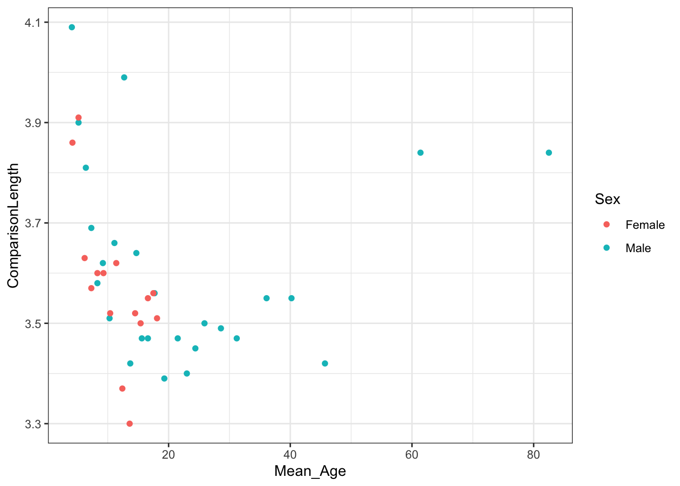

Figure 1.11: You won't have a caption. We will cover that later!

End of Comparison!