Lab 13 Continuing the GLM: Two-factor designs

13.1 Overview

For the past couple of weeks we have been building our understanding of the General Linear Model and in particular how it applies to a one-factor between-subjects ANOVA. Remember this is the scenario where you have one IV (categorical) and one DV (continuous) and you want to know if there is a significant effect at the different levels of your factor; where factor is another name for variable (or IV) and level is another name for condition (or group). We started out with the decomposition matrix, calculated our sums of squares, and from there our F-value to determine if there was a significant effect. One thing that is really worth keeping in mind is that the ANOVA is an omnibus test in that it tells you there is a significant effect of that factor, but it doesn't specifically say in which way is that effect manifested; you always have to do a little work there to tease out the pattern of the effect. Say for instance you test a one-way ANOVA on three animal categories on some test (dogs, cats, gerbils). The ANOVA will tell you if there is an overall effect (or difference between groups) but you need to do a little work to find out is the difference between cats and dogs, dogs and gerbils, etc etc. But more on that another time.

One-way ANOVAs are great when you only have one IV but the really useful thing about ANOVAs, and the GLM really, is that it can handle much more complex situations; which we are going to look at a little today. You were asked to read up on Chapter 4 of Miller and Haden (2013) looking at two-factor, between-subjects designs. This is the scenario where you have two factors (IVs) and it is different people in each condition. For example, say your IVs were people who can/can't juggle, and people who do/don't have pets. You have 4 groups here as you have people who can juggle and have pets, people who can't juggle and have pets, people who can juggle and don't have pets, and people who can't juggle and who don't have pets (how sad!!!). This would be an example of a two-way between-subjects factorial ANOVA (also a 2x2 ANOVA). And it is this scenario that we will be looking at today.

The goals of this chapter are to:

1. extend our knowledge of ANOVAs and GLMs to deal with two factors between-subject designs.
2. understand the concepts of and calculate main effects and interactions.
3. be able to plot and interpret data from factorial ANOVAs.

13.2 PreClass Activity

Only one chapter to read this week. Some of the terms will be familiar but some novel so remember to take notes and think of examples which would use the same design but in a different scenario. Once you have read the chapter, try the suggested exercise from the chapter and then the MCQs below to see if you are following things correctly. Anything you are unsure of, post questions on the forum or ask them in the lab.

13.2.1 Read

Chapter

Read Chapter 4 of Miller and Haden (2013) and try to understand the situation where you have two factors with at least two levels each. In this lab we will look at interactions.

13.2.2 TRY

Test your understanding of Miller and Haden (2013) Chapter 4

1. To test your understanding, work through Computational Exercise #1 in Section 4.9 of Miller and Haden - the answer is in Section 4.10 so check your working but be sure to work through the example first. The concept of interactions should be familiar to you from your statistics lectures this semester.

2. Try these short MCQs on two factor, between-subjects designs:

3. A 2x2 factorial design contains how many cells? twofoursixeightwho do we appreciate!

4. What effect is / effects are tested in a 2x2 ANOVA with factors A and B? the main effects of A and B, and the AB interactiononly the main effects of A and Bonly the AB interactiona correlation between A and B

5. What is a marginal mean? the mean DV at a given level of one factor, averaged over the levels of the other factorsthe mean DV at a given level of one factor, at a particular level of the other factora mean that is nearly statistically significanta mean defined based on marginal likelihood

6. What is a cell mean? the mean DV at a given level of one factor, averaged over the levels of the other factorsthe mean DV at a given level of one factor, at a particular level of the other factora mean that is nearly statistically significanta mean defined based on marginal likelihood

7. A statistical test for a main effect tests the null hypothesis that simple effects in the sample are equivalentsimple effects in the population are equivalentsample marginal means are equivalentpopulation marginal means are equivalent

8. A statistical test for an interaction tests the null hypothesis that the effect of one factor is constant across the levels of the other in the populationthe effect of one factor is constant across the levels of the other in the samplesample marginal means are equivalentpopulation marginal means are equivalent

If you are not sure about the above questions, go back and read the chapter and make sure you understand the difference between a main effect (the effect at one of the IVs) and the interaction (the effect of one factor dependent on the levels of the other factor). Those are the key elements to really wrap your head around in a factorial ANOVA.

Note: factorial ANOVAs can get really complex with three, four, or more IVs, so when writing about one, it is often good to state something like two-way (meaning two IVs) or three-way (meaning three IVs) etc. Be clear for your reader.

Job Done - Activity Complete!

13.3 InClass Activity

13.3.1 Estimation equations and decomposition matrix

We will start today by working with a decomposition matrix for a two-way between-subjects ANOVA and then finish by using the afex::aov_ez() function to show you how you might practically carry out this analysis.

Consider the data below from a 2x2 between-subjects design with 3 observations per cell. Keep in mind that each cell is a particular combination of levels of A and B, and each value in a cell, in this instance, is a unique participant.

Table 13.1: Data for today's example

	B1	B2
A1	74, 65, 77	70, 74, 66
A2	67, 67, 64	78, 78, 84

The decomposition matrix for these data is shown below; however, rather unfortunately for us, it is missing the columns AB_ij (\(\hat{A}_{ij}\)) and err (\(\widehat{S(AB)}_{ijk}\)) which we will need to calculate to complete our analysis.

Here is a little recap of the columns (plus the two we will add):

• \(i\) - the first factor (here with two levels)
• \(j\) - the second factor (again here with two levels)
• \(k\) - the participant number within that \(ij\) combination
• \(Y_{ijk}\) - a participants score on a DV
• \(\mu\) (mu) - the overall grand mean (or baseline effect)
• \(A_i\) - the effect of the first factor \(i\)
• \(B_j\) - the effect of the second factor \(j\)
• \(\hat{AB}_{ij}\) - the effect of the AB interaction
• \(\widehat{S(AB)}_{ijk}\) - the effect of within-group variability or error, err

Table 13.2: Incomplete Decomposition Matrix

i	j	k	Y_ijk	mu	A_i	B_j
1	1	1	74	72	-1	-3
1	1	2	65	72	-1	-3
1	1	3	77	72	-1	-3
1	2	1	70	72	-1	3
1	2	2	74	72	-1	3
1	2	3	66	72	-1	3
2	1	1	67	72	1	-3
2	1	2	67	72	1	-3
2	1	3	64	72	1	-3
2	2	1	78	72	1	3
2	2	2	78	72	1	3
2	2	3	84	72	1	3

The code to create the above matrix is in the solutions at the end of this chapter in case you want to create the matrix yourself as practice. If not, copy and paste the code from the solutions into a code chunk of an R Markdown file or into an R script (and make sure you also load tidyverse so that you can use the dplyr functions and pipes.)

Run the code and look at decomp to confirm to yourself that it worked. Note the use of the group_by() function so that the values calculated with in mutate() are only calculated for each group.

13.3.2 Adding the missing columns

Once you understand the table and code, try writing code to add the two missing columns to our matrix. Store the resulting table in decomp2.

Here are some hints but again the code is in the solutions if you can't quite get it - but remember, to paraphrase Dumbledore: "Help will always be given at Glasgow to those that look for it."

Hints:

• AB_ij - (\(\hat{A}_{ij}\)) - is what is left of the mean value of all participants in that group once you have removed the effect of the grand mean, the effect of factor one, and the effect of factor two
• err - (\(\widehat{S(AB)}_{ijk}\)) - is what is left from an individual's score after removing the effect of the grand mean, the effect of factor A, the effect of factor B, and the interaction effect.

13.3.3 Understanding the two-factor decomposition matrix

If you have performed the above steps correctly, then the decomp matrix should now look like

Table 13.3: The complete decomposition matrix

i	j	k	Y_ijk	mu	A_i	B_j	AB_ij	err
1	1	1	74	72	-1	-3	4	2
1	1	2	65	72	-1	-3	4	-7
1	1	3	77	72	-1	-3	4	5
1	2	1	70	72	-1	3	-4	0
1	2	2	74	72	-1	3	-4	4
1	2	3	66	72	-1	3	-4	-4
2	1	1	67	72	1	-3	-4	1
2	1	2	67	72	1	-3	-4	1
2	1	3	64	72	1	-3	-4	-2
2	2	1	78	72	1	3	4	-2
2	2	2	78	72	1	3	4	-2
2	2	3	84	72	1	3	4	4

So let's now make sure we understand the table that we have and that we can pinpoint different elements of it by answering the following questions. The solutions are at the end of the chapter.

1. From the options, what was the DV-value of participant \(Y_{212}\)? 64656667

2. Type in the value of \(SS_{B}\):

3. Type in the value of \(SS_{error}\) is:

4. Type in the value of \(MS_{B}\) is:

5. Type in the value of \(MS_{error}\) (to one decimal places) is:

6. The value of \(F_{B}\) (the F-ratio for the main effect of B) to 3 decimal places is:

7. The numerator and denominator degrees of freedom associated with this \(F\) ratio are and respectively

8. The \(p\) value associated with this F ratio to three decimal places is (HINT: ?pf):

13.3.4 Get your data ready for analysis

It is excellent that you now understand a decomposition matrix and how it relates to an F-ratio. In reality however, rarely will you ever derive a decomposition matrix by hand; the point was to improve your understanding of the calculations behind an ANOVA.

Let's continue using the simulated data from above and run through the analysis steps we would normally follow. But first, let's put it in a more useful format.

The first thing we might want to do is to add columns that more clearly indicate the levels of our two factors. Right now the levels of A are represented by i and the levels of B are represented by j. But the data should really look more like this below:

Table 13.4: Converted Decomposition Matrix

id	A	B	Y_ijk
1	A1	B1	74
2	A1	B1	65
3	A1	B1	77
4	A1	B2	70
5	A1	B2	74
6	A1	B2	66
7	A2	B1	67
8	A2	B1	67
9	A2	B1	64
10	A2	B2	78
11	A2	B2	78
12	A2	B2	84

We will need the id column (a unique value for each participant) for when we run afex::aov_ez() later.

Again the code to convert decomp into this table (named dat) is in the solutions at the end of the chapter and you can use it if you like, but if you want to practice your skills first and convert the table yourself, that is also fine. Don't spend too long on it though as it is more the output we want to look at. So if you are stuck, copy the code and run it in your session. We'll be working with the new table dat for the remaining exercises.

13.3.5 Visualizing 2x2 designs: The interaction plot

A critical part of data analysis is visualization. When dealing with factorial data, one of the most important visualizations is the interaction plot showing the cell means. You have already seen some of these in the Miller and Haden chapter and in the previous labs.

Remember that before you can make an interaction plot, you need to calculate the cell means.

• First create a table called cell_means with the cell means stored in the column m. HINT - think group_by and summarise to leave three columns only, each with 4 rows. For example, one row will show A, A, mean-value

• Next, reproduce the plot below. Don't look at the solution below until you've really tried! You will need two geoms: one to draw the points, one to draw the lines. And think about what is your x and y axes and how do you group the lines.

## `summarise()` has grouped output by 'A'. You can override using the `.groups` argument.

Figure 13.1: Interaction plot

13.3.6 Running a 2x2 between-subjects ANOVA with aov_ez

Excellent! So we have a figure now! In reality, you would want to embellish this figure to make it look more professional, add some error bars, make sure the whole of the y-axis is shown, give proper names to the factors and levels, but it will do for now. You also want to look at the figure and think about what it is telling you. Do you think there will be:

1. A main effect of Factor A?
2. A main effect of Factor B?
3. An interaction between Factors A and B?

To some degree these are the three basic hypotheses laid out in any two-way ANOVA. To answer these you can think about:

1. Are the means of \(A_1\) and \(A_2\) different, disregarding the effect of Factor B?
2. Are the means of \(B_1\) and \(B_2\) different, disregarding the effect of Factor A?
3. Are the means of \(A_1\) and \(A_2\) influenced by the effect of Factor B? What do non-parallel (or crossing lines) suggest about an interaction?

Looking at the figure you might suggest, no main effect of A, no main effect of B, but that there is an interaction between A and B. Let's test this using the afex::aov_ez() function!

• Perform the 2x2 ANOVA on dat and store the output in result.
  • Try not to look at the solution until you have tried the ?aov_ez to see how to add more than one condition of the same design.
  • a second hint is that both factors are "between", so you want to focus on adding a second "between" condition
  • set type = 3

We have also placed a short summary of the output of the ANOVA below to give you an idea of the outcome. Think about the outcome for a moment or two before having a go at writing one out and then look at the summary to compare.

A two-way between-subjects factorial ANOVA was conducted. A significant interaction was found between Factor A and Factor B, F(1, 8) = 10.97, p = .011, ges = .59. Furthermore, a main effect of Factor B was found, F(1, 8) = 6.17, p = .038, ges = .44, which showed that the mean of \(B_2\) (M = 75) was significantly larger than the mean of \(B_1\) (M = 69). However, no main effect of Factor A was found, F(1, 8) = 0.686, p = .43, ges = .08. The mean of \(A_1\) (M = 71) was similar to the mean of \(A_2\) (M = 73).

So it turns out we were sort of right and sort of wrong. There was no main effect of Factor A as we predicted. The means at \(A_1\) and \(A_2\) are very similar when you disregard the effect of Factor B. However, there actually was a main effect of Factor B; i.e. there was a significant difference between the means of \(B_1\) and \(B_2\) when you disregard the effect of Factor A. And finally, we predicted that there would be a significant interaction and there was one because the effect of Factor A is modulated by Factor B, and vice versa.

One thing to point out here, when there are only two conditions in a factor and there is a significant main effect of that Factor (in this example Factor B) then to further qualify that effect you simply have to say which of the two conditions was bigger than the other! Group 2 bigger than Group 1 or Group 1 bigger than Group 2. When there is more than two conditions in a factor (e.g. three) or in the interaction, it is not that straightforward and you need to do further comparisons such as pairwise comparisons, t-test, simple main effects, or TUKEY HSDs, to tease those effects a part. We will cover more of that in the lecture series.

13.3.7 App: Understanding main effects and interactions

If time permits (or on your own time), check out the accompanying shiny app, below, on main effects and interactions or by clicking here. This allows you to move sliders and change the sizes of main effects / interactions and see how this affects cell means and effect decompositions. This will help sharpen your intuitions about these concepts.

Figure 4.11: Main Effects and Interactions App

Job Done - Activity Complete!

One last thing:

Before ending this section, if you have any questions, please post them on the available forums or speak to a member of the team. Finally, don't forget to add any useful information to your Portfolio before you leave it too long and forget. Remember the more you work with knowledge and skills the easier they become.

13.4 Test Yourself

This is a formative assignment meaning that it is purely for you to test your own knowledge, skill development, and learning, and does not count towards an overall grade. However, you are strongly encouraged to do the assignment as it will continue to boost your skills which you will need in future assignments. You will be instructed by the Course Lead on Moodle as to when you should attempt this assignment. Please check the information and schedule on the Level 2 Moodle page.

Lab 13: Two-Factor ANOVA: Perspective-Taking in Language Comprehension

In order to complete this assignment you first have to download the assignment .Rmd file which you need to edit for this assignment: titled GUID_Level2_Semester2_Lab4.Rmd. This can be downloaded within a zip file from the below link. Once downloaded and unzipped you should create a new folder that you will use as your working directory; put the .Rmd file in that folder and set your working directory to that folder through the drop-down menus at the top. Download the Assignment .zip file from here or on Moodle.

Background: Perspective-Taking in Language Comprehension

For this assignment, you will be looking at real data from Experiment 2 of Keysar, Lin, and Barr (2003), "Limits on Theory of Mind Use in Adults", Cognition, 89, 29--41. This study used eye-tracking to investigate people's ability to take another's perspective during a kind of communication game. (The data that you will be analysing, while real, did not appear in the original report.)

The communication game that participants played was as follows. Each participant sat at a table opposite a confederate participant (a stooge from the lab who pretended to be a naive participant). Between the two participants was an upright set of shelves (see figure below). The participants played a game in which the real participant was assigned the role of the "matcher" and the confederate the role of the "director". The director was given a picture with a goal state for the grid, showing how the objects needed to be arranged. However, the director was not allowed to touch the objects. To get the objects in their proper places, the director needed to give instructions to the matcher to move the objects. For example, the director might say, "take the red box in the top corner and move it down to the very bottom row," and the matcher would then perform the action. The matcher's eye movements were tracked as they listened to and interpreted the director's instructions.

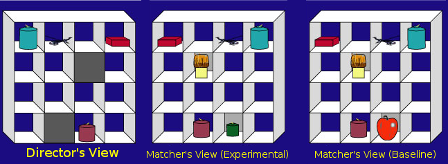
Figure 13.2: Director-Matcher Viewpoints from Keysar, Lin, and Barr (2003)

To investigate perspective taking, the instructions given by the director were actually scripted beforehand in order to create certain ambiguities. Most of the objects in the grid, such as the red box, were mutually visible to both participants (i.e., visible from both sides of the grid). However, some of objects, like the brush and the green candle, were occluded from the director's view; the matcher could see them, but had no reason to believe that the director knew the contents of these occluded squares, and thus had no reason to expect her to ever refer to them. However, sometimes the director would refer to a mutually visible object using a description that also happened to match one of the hidden objects. For instance, the director might instruct the matcher to "pick up the small candle." Note that for the director, the small candle is the purple candle. A given matcher would see this grid in one of two conditions: In the Experimental condition, the matcher saw an additional green candle in a hidden box that was even smaller than the purple candle (see middle panel of the above figure). This object was called a "competitor" because it matched the description of the intended referent (the purple candle). In the Baseline condition, the green candle was replaced with an object that did not match the director's description, such as an apple. These ambiguous situations provided the main data for the experiment, and in total there were eight different grids in the experiment that presented analogous situations to the example above.

A previous eye-tracking study by the same authors had found the presence of the competitors severely confused the matchers, suggesting that people were surprisingly egocentric---they found it hard to ignore "privileged" information when interpreting another person's speech. For example, when the director said to "pick up the small candle," they spent far more time looking at a hidden green candle than a hidden apple, even though neither one of these objects, being hidden, was a viable referent. We refer to the difference in looking time as the 'egocentric interference effect'.

Experiment 2 by Keysar, Lin, and Barr aimed to follow up on this finding. In the previous article, the matcher had reason to believe that the director was merely ignorant of the identity of the hidden objects. But what would happen if the matcher was given reason to believe that the director actually had a false belief about the hidden object? For example, would the matcher experience less egocentric interference if he or she had reason to think that the director thought that the hidden candle was a toy truck?

To test this, half of the participants were randomly assigned to a false belief condition, where the matcher was led to believe that the director had a false belief about the identity of the hidden object; the other half participated in the ignorance condition, where as in previous experiments, they were led to believe that the director simply did not know what was in the hidden squares.

There were 40 participants in this study, 20 in the false belief condition, and 20 in the ignorance condition. There were also an equal number of male and female participants in the study. To spoil the plot a bit, Keysar, Lin and Barr did not find any effect of condition on looking time. However, they did not consider sex as a potential moderating variable. Thus, we will explore the effects of ignorance vs. false belief on egocentric interference, broken down by the sex of the matcher.

Before starting lets check:

1. The .csv file is saved into a folder on your computer and you have manually set this folder as your working directory.

2. The .Rmd file is saved in the same folder as the .csv files. For assessments we ask that you save it with the format GUID_Level2_Semester2_Lab4.Rmd where GUID is replaced with your GUID. Though this is a formative assessment, it may be good practice to do the same here.

13.4.1 Task 1A: Libraries

• In today's assignment you will need both the tidyverse and ez packages. Enter code into the t1A code chunk below to load in both of these libraries.

# load in the packages

13.4.2 Task 1B: Loading in the data

• Use read_csv() to replace the NULL in the t1B code chunk below to load in the data stored in the datafile keysar_lin_barr_2003.csv. Store the data in the variable dat. Do not change the filename of the datafile.

dat <- NULL

Take a look at your data (dat) in the console using glimpse() or View(), or just display it by typing in the name. You will see the following columns:

variable	description
subject	unique identifier for each subject
sex	whether the subject was male or female
condition	what condition the subject was in
looktime	egocentric interference

We have simplified things from the original experiment by collapsing the baseline vs. experimental conditions into a single DV. Our DV, egocentric interference, is the average difference in looking time for each subject (in milliseconds per trial) for hidden competitors (e.g., small candle) versus hidden non-competitors (e.g., apple). The larger this number, the more egocentric interference the subject experienced.

13.4.3 Task 2: Calculate cell means

Today we are going to focus on just the main analysis and write-up, and not the assumptions, but as always before running any analysis you should check that your assumptions hold.

One of the elements we will need for our write-up is some descriptives. We want to start by creating some summary statistics for the four conditions. Remember, two factors (sex and condition) with 2 levels each (sex: female vs. male; condition: false belief vs. ignorance) will give you four conditions, and as such in our summary table, four cells created by factorially combining sex and condition.

• Replace the NULL in the t2 code chunk below to create the four cells created by factorially combining sex and condition, calculating the mean and standard deviation for each cell.
  • Store the descriptives in the tibble called cell_means
  • Call the column for the mean m and the column for the standard deviation sd.
  • Your table should have four rows and four columns as shown below but with your values replacing the XXs
  • Follow the case and spelling exactly.

cell_means <- NULL

sex	condition	m	sd
female	false belief	XX	XX
female	ignorance	XX	XX
male	false belief	XX	XX
male	ignorance	XX	XX

13.4.4 Task 3: Marginal means for sex

We will also need to have some descriptives where we just look at the means of a given factor; the marginal means - the means of the levels of one factor regardless of the other factor.

• Replace the NULL in the t3 code chunk below to calculate the marginal means and standard deviations for the factor sex.
  • Store these descriptives in the tibble marg_sex
  • Call the column for the mean m and the column for the standard deviation sd.
  • Your table should have two rows and three columns as shown below but with your values replacing the XXs
  • Follow the case and spelling exactly.

marg_sex <- NULL

sex	m	sd
female	XX	XX
male	XX	XX

13.4.5 Task 4: Marginal means for condition

And now do the same for condition.

• Replace the NULL in the t4 code chunk below to calculate the marginal means and standard deviations for the factor, condition
  • Store these descriptives in the tibble marg_cond
  • Call the column for the mean m and the column for the standard deviation sd.
  • Your table should have two rows and three columns as shown below but with your values replacing the XXs
  • Follow the case and spelling exactly.

marg_cond <- NULL

condition	m	sd
false belief	XX	XX
ignorance	XX	XX

13.4.6 Task 5: Interaction plot

And finally we are going to need a plot. When you have two factors, you want to show both factors on the plot to give the reader as much information as possible and save on figure space. The best way to do this is through some sort of interaction plot as shown in the lab. It is really a lot easier than it looks and it only requires you to think about setting the aes by the different conditions.

• Insert code into the t5 code chunk below to replicate the figure shown to you.
  • Pay particular attention to labels, axes dimensions, color and background.
  • Note that the figure must appear when your code is knitted.
• Note: The figure below is a nice figure but should really have error bars on it if I was including it in an actual paper. Including the error bars may help in clarifying the descriptive statistics and you will see that here, although the means are different, there is huge overlap in terms of error bars which may indicate no overall effect.

# to do: something with ggplot to replicate the figure

## `summarise()` has grouped output by 'sex'. You can override using the `.groups` argument.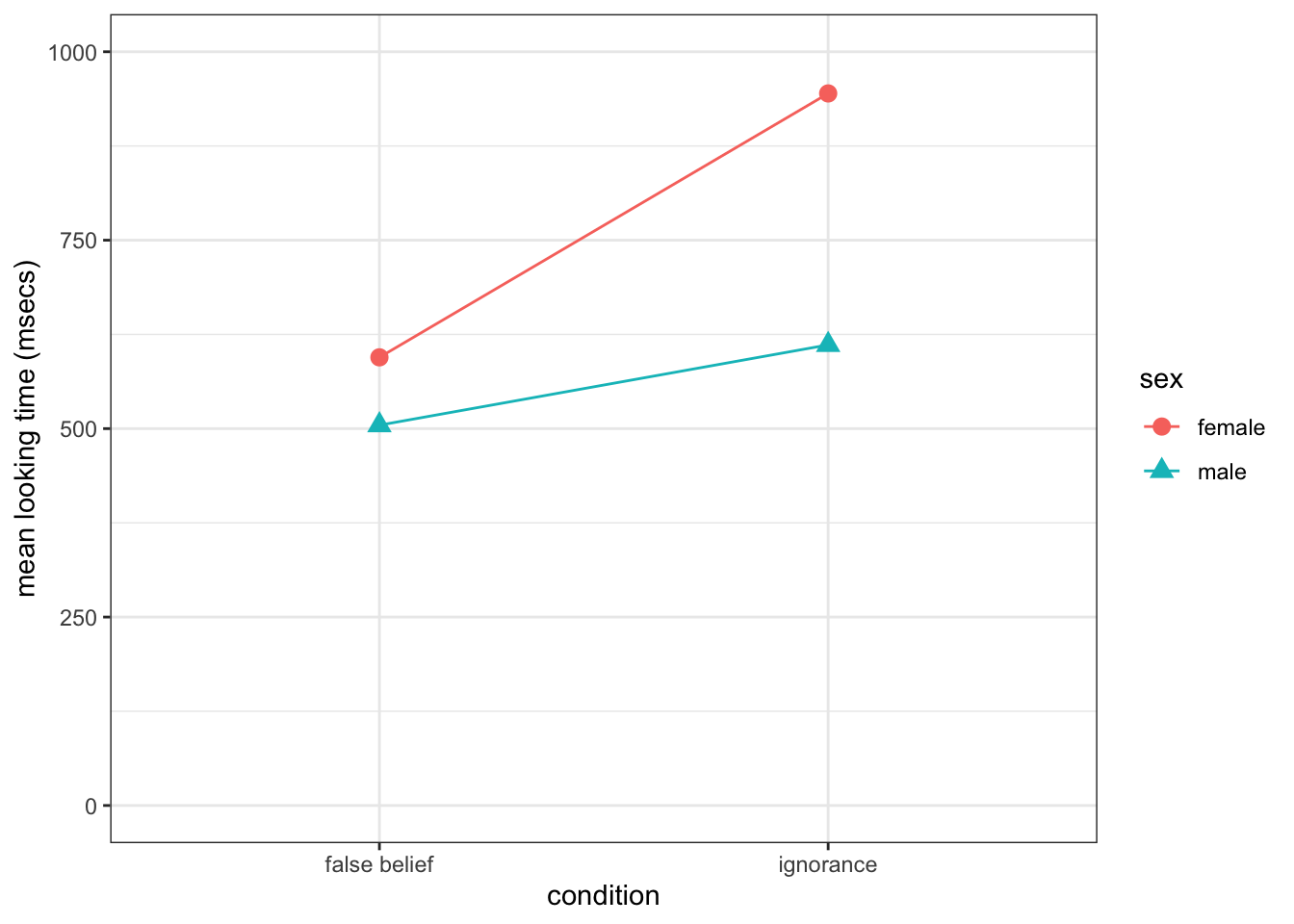

Figure 13.3: Replicate this Figure

13.4.7 Task 6: Recap Question 1

Thinking about the above information, one of the below statements would be an acceptable hypothesis for the interaction effect of sex and condition, but which one:

• In the t6 code chunk below, replace the NULL with the number of the statement below that best summarises this analysis. Store this single value in answer_t6

1. We hypothesised that there will be a significant difference between males and females in egocentric interference (mean looking time (msecs)) regardless of condition.
2. We hypothesised that there will be a significant difference between participants in the false belief condition and those in the ignorance condition in terms of egocentric interference (mean looking time (msecs)) regardless of sex of participant.
3. We hypothesised that there would be a significant interaction between condition and sex of participant on egocentric interference (mean looking time (msecs))
4. We hypothesised that there will be no significant difference between males and females in egocentric interference (mean looking time (msecs)) regardless of condition but that there would be a significant difference between participants in the false belief condition and those in the ignorance condition in terms of egocentric interference (mean looking time (msecs)) regardless of sex of participant.

answer_t6 <- NULL

13.4.8 Task 7: Recap Question 2

Thinking about the above information, one of the below statements is a good description of the marginal means for sex, but which one:

• In the t7 code chunk below, replace the NULL with the number of the statement below that best summarises this analysis. Store this single value in answer_t7

1. The female participants have an average longer looking time (M = 777.98, SD = 911.53) than the male participants (M = 555.04, SD = 707.81) which may suggest a significant main effect of sex.
2. The female participants have an average shorter looking time (M = 777.98, SD = 911.53) than the male participants (M = 555.04, SD = 707.81) which may suggest a significant main effect of condition.
3. The female participants have an average shorter looking time (M = 777.98, SD = 911.53) than the male participants (M = 555.04, SD = 707.81) which may suggest a significant main effect of sex.
4. The female participants have an average longer looking time (M = 777.98, SD = 911.53) than the male participants (M = 555.04, SD = 707.81) which may suggest a significant main effect of condition.

answer_t7 <- NULL

13.4.9 Task 8: Recap Question 3

Thinking about the above information, one of the below statements is a good description of the marginal means for condition, but which one:

• In the t8 code chunk below, replace the NULL with the number of the statement below that best summarises this analysis. Store this single value in answer_t8

1. The participants in the false belief group had an average longer looking time (M = 549.58, SD = 775.91) than the participants in the ignorance group (M = 749.58, SD = 861.23), which may suggest a significant main effect of condition.
2. The participants in the false belief group had an average shorter looking time (M = 549.58, SD = 775.91) than the participants in the ignorance group (M = 749.58, SD = 861.23), which may suggest a significant main effect of condition.
3. The participants in the false belief group had an average longer looking time (M = 549.58, SD = 775.91) than the participants in the ignorance group (M = 749.58, SD = 861.23), which may suggest a significant main effect of sex.
4. The participants in the false belief group had an average shorter looking time (M = 549.58, SD = 775.91) than the participants in the ignorance group (M = 749.58, SD = 861.23), which may suggest a significant main effect of sex.

answer_t8 <- NULL

13.4.10 Task 9: Running the factorial ANOVA

Great, so we have looked at our descriptives and thought about what effects there might be. What we need to do now is run the ANOVA using the aov_ez() function. The ANOVA we are going to run is a two-way between-subjects ANOVA because both conditions are between-subjects variables. You may need to refer back to the lab or to have a look at the help on aov_ez() to see how to add a second variable/factor.

• Replace the NULL in the t9 code chunk below to run this two-way between-subjects ANOVA.
  • Look at the inclass for guidance. You need the data, the dv, the two between condition, and the participant id.
  • Set the type to type = 3
  • Do not tidy() the output. Do nothing to the output other than store it in the variable named mod (note: technically it will store as a list).
  • You will see in red in the output that the code will convert the conditions to factors automatically, and set the contrasts. This is fine.

mod <- NULL

13.4.11 Task 10: Interpreting the ANOVA output Question

Thinking about the above information, one of the below statements is a good summary of the outcome ANOVA, but which one:

• In the t10 code chunk below, replace the NULL with the number of the statement below that best summarises this analysis. Store this single value in answer_t10

1. There is a significant main effect of sex, but no main effect of condition and no interaction between condition and sex.
2. There is a significant main effect of condition, but no main effect of sex and no interaction between condition and sex.
3. There is no significant main effect of sex or condition and there is no significant interaction between condition and sex.
4. There is a significant main effect of sex, a significant main effect of condition, and a significant interaction between condition and sex.

answer_t10 <- NULL

13.4.12 Task 11: Report your results

Write a paragraph reporting your findings. NOTE: You can use inline code to report the \(F\) values, but note that you cannot use broom::tidy() for objects created by ezANOVA(). Here is a hint: mod$ANOVA gives you a table of your results (ezANOVA() returns a list with two elements; mod$ANOVA returns the element of the list called ANOVA that has the results). You can pull() and pluck() whatever you need from this table.

Write your summary between the two green lines shown in the Assignment file.

Job Done - Activity Complete!

Well done, you are finished! Now you should go check your answers against the solution file which can be found on Moodle. You are looking to check that the resulting output from the answers that you have submitted are exactly the same as the output in the solution - for example, remember that a single value is not the same as a coded answer. Where there are alternative answers it means that you could have submitted any one of the options as they should all return the same answer. If you have any questions please post them on the forums

See you in the next lab!

13.5 Solutions to Questions

Below you will find the solutions to the questions for the Activities for this chapter. Only look at them after giving the questions a good try and speaking to the tutor about any issues.

13.5.1 InClass Activities

13.5.1.1 Estimation equations and decomposition matrix

Creating the Decomposition Matrix

decomp <- tibble(i = rep(1:2, each = 6),
                 j = rep(rep(1:2, each = 3), times = 2),
                 k = rep(1:3, times = 4),
                 Y_ijk = c(74, 65, 77, 70, 74, 66, 67, 67, 64, 78, 78, 84)) %>%
    mutate(mu = mean(Y_ijk)) %>% # calculate mu
    group_by(i) %>% 
    mutate(A_i = mean(Y_ijk) - mu) %>% # calculate A_i
    group_by(j) %>% 
    mutate(B_j = mean(Y_ijk) - mu) %>% # calculate B_j
    ungroup()

Return to Task

13.5.1.2 Adding the missing columns

decomp2 <- decomp %>%
  group_by(i, j) %>%
  mutate(AB_ij = mean(Y_ijk) - mu - A_i - B_j) %>%
  ungroup() %>%
  mutate(err = Y_ijk - mu - A_i - B_j - AB_ij)

Return to Task

13.5.1.3 Understanding the two-factor decomposition matrix

Q1

The DV value of participant \(Y_{212}\) or the 2nd Participant in \(I_2\), \(J_1\), is 67

Q2

The Sums of Squares of Factor B is 108

Q3

The Sums of Squares of the Error is 140

Q4

The \(MS_{B}\) is 108

Q5

The \(MS_{error}\) (to one decimal places) is 17.5

Q6

The F-ratio for the main effect of B to 3 decimal places is 6.171

Q7

The numerator and denominator degrees of freedom associated with this \(F\) ratio are 1 and 8 respectively

Q8

And based on pf(fratio, 1,8, lower.tail = FALSE) the \(p\)-value associated with this F ratio to three decimal places is 0.038 or .038

Return to Task

13.5.1.4 Get your data ready for analysis

dat <- decomp %>%
  mutate(A = paste0("A", i),
         B = paste0("B", j),
         id = row_number()) %>%
  select(id, A, B, Y_ijk)

Return to Task

13.5.1.5 Visualizing 2x2 designs: The interaction plot

Creating the Cell means

cell_means <- dat %>%
  group_by(A, B) %>%
  summarise(m = mean(Y_ijk))

## `summarise()` has grouped output by 'A'. You can override using the `.groups` argument.

Reproducing the Plot

ggplot(cell_means, aes(A, m, group = B, shape = B, color = B)) +
  geom_point(size = 3) +
  geom_line()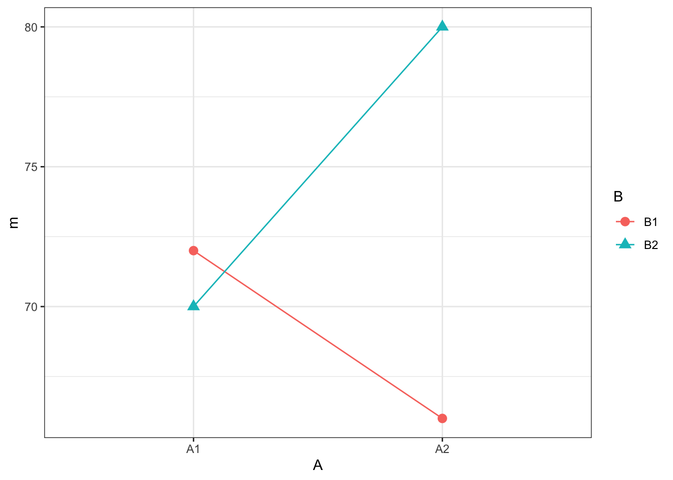

Figure 13.4: The plot that the code gives

Easter Egg Figure Solution

The plot above is functional but sometimes you want something a bit more communicative. It is worth working on your figures so, here is an example of what you can think about for your report. Remember to look back through previous labs and homework as well (Semester 1: Lab 3, Lab 7, Lab 6, Lab 5 & 9 assignments, for instance) to see how figures can be improved.

The code below adds another few dimensions to the above figure. Copy and run the code in your Rmd, knitting it to HTML, and play with the different parts to see what they do. We have changed the legends to be more descriptive and to have more readable text, fixed the scale for the vertical axis, made the figure black and white without a box, we also added 95% confidence intervals and a figure caption.

There are of course various ways to do these changes, in particular the caption, but this is an option.

Note: This will only run if you have the tibble dat from earlier in this worksheet

cell_means1 <- dat %>%
group_by(A, B) %>%
summarise(m = mean(Y_ijk),
          n = n(),
          sd_scores = sd(Y_ijk),
          ste_scores = sd_scores/sqrt(n),
          ci = 1.96 * ste_scores)

## `summarise()` has grouped output by 'A'. You can override using the `.groups` argument.

ggplot(cell_means1, aes(A, m, group = B)) +
  geom_point(aes(shape = B), size = 3) +
  geom_line() +
  geom_errorbar(aes(ymin = m - ci, ymax = m + ci), 
                width = 0.05, 
                size = .5) +
  coord_cartesian(ylim = c(0,100)) +
  labs(x = "Groups in Factor A", 
       y = "Mean Scores", 
       caption = "Figure 1. Mean scores from the example data for the two-way \nbetween-subjects design ANOVA. Error bars indicate 95% \nconfidence intervals.") +
  scale_shape_discrete("Groups in Factor B") +
  theme_classic() +
  theme(axis.text.x = element_text(size = 12),
        axis.text.y = element_text(size = 12),
        axis.title = element_text(size = 14),
        legend.title = element_text(size = 14),
        legend.text = element_text(size = 14),
        plot.caption  = element_text(size = 14, hjust = 0))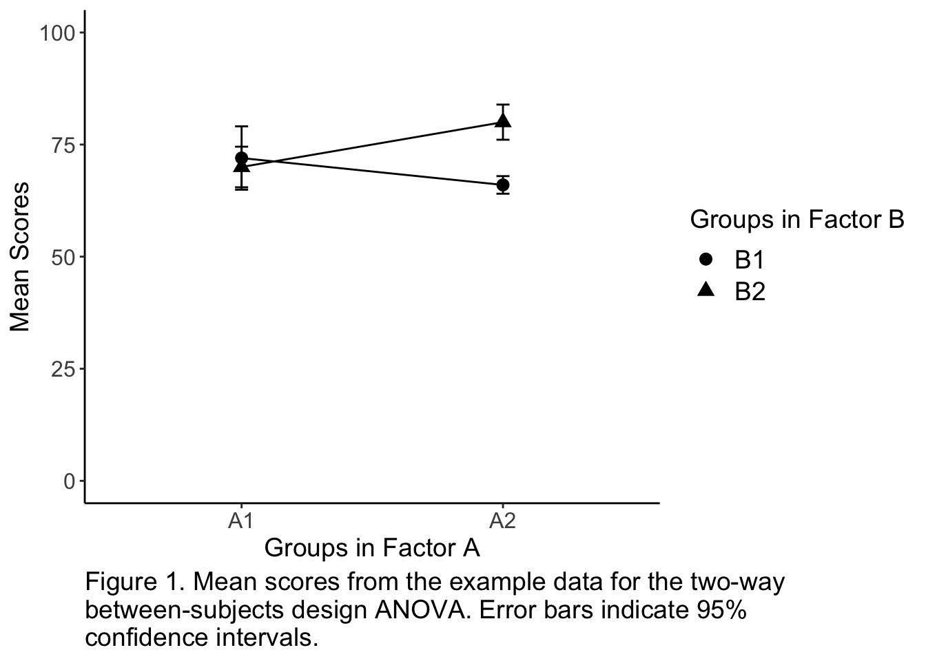

Figure 13.5: A nice figure example

Return to Task

13.5.1.6 ANOVA Using aov_ez

The code

result <- aov_ez(data = dat, 
                  dv = "Y_ijk", 
                  id = "id",
                  type = 3,
                  between = c("A", "B"))

## Converting to factor: A, B

## Contrasts set to contr.sum for the following variables: A, B

result$anova_table

	num Df	den Df	MSE	F	ges	Pr(>F)
A	1	8	17.5	0.6857143	0.0789474	0.4316340
B	1	8	17.5	6.1714286	0.4354839	0.0378608
A:B	1	8	17.5	10.9714286	0.5783133	0.0106614

The output

• Using the anova_table within the output, i.e. result$anova_table, would show us:

Table 13.5: The ANOVA output

	num Df	den Df	MSE	F	ges	Pr(>F)
A	1	8	17.5	0.686	0.079	0.432
B	1	8	17.5	6.171	0.435	0.038
A:B	1	8	17.5	10.971	0.578	0.011

• Alternatively, using the Anova within the output, i.e. result$Anova, would show us the Sums of Squares as well:

Table 13.6: The ANOVA output

	Sum Sq	Df	F value	Pr(>F)
(Intercept)	62208	1	3554.743	0.000
A	12	1	0.686	0.432
B	108	1	6.171	0.038
A:B	192	1	10.971	0.011
Residuals	140	8	NA	NA

Return to Task

13.5.2 Test Yourself Activities

13.5.2.1 Task 1A: Libraries

• In today's assignment you will need both the tidyverse and ez packages.

library(afex)
library(tidyverse)

Return to Task

13.5.2.2 Task 1B: Loading in the data

• Remember to use read_csv() to load in the data.

dat <- read_csv("keysar_lin_barr_2003.csv")

Return to Task

13.5.2.3 Task 2: Calculate cell means for the cell means.

• The code below will give the table shown.

cell_means <- dat %>%
  group_by(sex, condition) %>%
  summarise(m = mean(looktime), sd = sd(looktime))

## `summarise()` has grouped output by 'sex'. You can override using the `.groups` argument.

sex	condition	m	sd
female	false belief	594.5833	899.1660
female	ignorance	944.6970	932.6990
male	false belief	504.5833	676.7338
male	ignorance	611.1111	778.0212

Return to Task

13.5.2.4 Task 3: Marginal means for sex

• The code below will give the table shown for the marginal means of sex.

marg_sex <- dat %>%
  group_by(sex) %>%
  summarise(m = mean(looktime), sd = sd(looktime))

sex	m	sd
female	777.9762	911.5331
male	555.0439	707.8138

Return to Task

13.5.2.5 Task 4: Marginal means for condition

• The code below will give the table shown for the marginal means of condition.

marg_cond <- dat %>%
  group_by(condition) %>%
  summarise(m = mean(looktime), sd = sd(looktime))

condition	m	sd
false belief	549.5833	775.9108
ignorance	794.5833	861.2306

Return to Task

13.5.2.6 Task 5: Interaction plot

• The code below will produce the shown figure.

ggplot(cell_means, aes(condition, m, shape = sex, group = sex, color = sex)) +
  geom_line() +
  geom_point(size = 3) +
  labs(y = "mean looking time (msecs)") +
  scale_y_continuous(limits = c(0, 1000)) + 
  theme_bw()

Figure 13.6: You should have produced a similar figure

Return to Task

13.5.2.7 Task 6: Recap Question 1

We want the alternative, not the null hypothesis here. So, an acceptable hypothesis for the interaction effect of sex and condition would be:

We hypothesised that there would be a significant interaction between condition and sex of participant on egocentric interference (mean looking time (msecs)).

As such the correct answer is:

answer_t6 <- 3

Return to Task

13.5.2.8 Task 7: Recap Question 2

A good description of the marginal means for sex would be:

The female participants have an average longer looking time (M = 777.98, SD = 911.53) than the male participants (M = 555.04, SD = 707.81) which may suggest a significant main effect of sex.

As such the correct answer is:

answer_t7 <- 1

Return to Task

13.5.2.9 Task 8: Recap Question 3

A good description of the marginal means for condition would be:

The participants in the false belief group had an average shorter looking time (M = 549.58, SD = 775.91) than the participants in the ignorance group (M = 749.58, SD = 861.23), which may suggest a significant main effect of condition.

As such the correct answer is:

answer_t8 <- 2

Return to Task

13.5.2.10 Task 9: Running the factorial ANOVA

• The code below will produce the shown ANOVA output

mod <- aov_ez(data = dat,
                   dv = "looktime", 
                   id = "subject",
                   type = 3,
                   between = c("condition", "sex"))

knitr::kable(mod$anova_table)

	num Df	den Df	MSE	F	ges	Pr(>F)
condition	1	36	692778.4	0.7487009	0.0203735	0.3926176
sex	1	36	692778.4	0.6442294	0.0175807	0.4274507
condition:sex	1	36	692778.4	0.2130405	0.0058830	0.6471716

Return to Task

13.5.2.11 Task 10: Interpreting the ANOVA output Question

A good summary of the outcome ANOVA would be:

There is no significant main effect of sex or condition and there is no significant interaction between condition and sex.

As such the correct answer is:

answer_t10 <- 3

Return to Task

13.5.2.12 Task 11: Report your results

There is no definitive way to write this paragraph but essentially your findings should report both main effects and the interaction, giving appropriate F outputs, e.g. F(1, 36) = .79, p = .38, and give some interpretation/qualification of the results using the means and standard deviations above, e.g. looking time was not significantly different between the false belief task (M = X, SD = XX) or the Ignorance task (M = XX, SD = XX). Something along the following would be appropriate:

A two-way between-subjects factorial ANOVA was conducted testing the main effects and interaction between sex (male vs. female) and condition (false belief vs. ignorance) on the average looking time (msecs) on a matching task. Results revealed no significant interaction (F(1, 36) = .21, p = .647) suggesting that there is no modulation of condition by sex of participant in this looking task. Furthermore, there was no significant main effect of sex (F(1, 36) = .64, p = .429) suggesting that male (M = 555.04, SD = 707.81) and female participants (M = 777.98, SD = 911.53) perform similarly in this task. Finally, there was no significant main effect of condition (F(1, 36) = .79, p = .38) suggesting that whether participants were given a false belief scenario (M = 594.58, SD = 775.91) or an ignorance scenario (M = 794.58, SD = 861.23) had no overall impact on their performance.

Return to Task

Chapter Complete!