Lab 4 Revisiting Probability Distributions
4.1 Overview
Probability is to some degree the cornerstone of any Psychological theory that is based on quantitative analysis. We establish an outcome (e.g. a difference between two events), then establish the probability of that outcome against some model or standard. Probability is important for quantifying the uncertainty in our conclusions. You will have already heard about probability in lectures/journal articles/etc but we will try to help you gain a deeper understanding of probability through the course of the next few chapters and in how we use it to make an inference about a population.
We will start by looking at some of the general ideas behind probability. We won't be using a lot of Psychology data or concepts here as it can be easier to understand probability first in everyday concrete examples. That said, whilst reading the examples, and trying them out, think about how they might relate to Psychology examples and be sure to ask questions.
This preclass is a bit of a read so take your time and try to understand it fully. Much of it will be familiar though from the PsyTeachR Grassroots book as it recaps some of the ideas. Also, there are no cheatsheets for this chapter as we will not be using a specific package. However you can make full use of the R help function (e.g. ?sample) when you are not clear on what a function does. Also, remember what we have said previously; do not be shy to do what we do and run a Google Search for finding out more about some of the stats concepts covered here. There are loads of videos and help pages out there with clear examples to explain difficult concepts.
In this chapter you will:
- Revise probability concepts that we discussed in the PsyTeachR Grassroots book
- Calculate probabilities
- Create probability distributions
- Make estimations from probability distributions.
The population is the whole group that you want to know something about - everyone or everything in that group. The sample is the part of the population that you are testing. The sample is always smaller than the population as it is unlikely that you would ever be able to test everyone in a population, but the sample should be representative of the population based on random sampling. This means that even though you are not using the whole population, the sample you are using represents the whole population because you randomly sampled people into it. If this is true, that the sample is representative of the population, then testing on the sample allows you to make some inference about the population; you infer a characteristic of the population from testing on the sample.
4.1.1 Discrete or Continuous Datasets
This is a short tutorial with just a couple of quick recap questions on how the level of measurement can alter the way you tackle probability - i.e. whether the data is discrete or continuous.
Quickfire Questions
Discrete data can only take specific/certain/exact values (e.g. groups, integers). For example, the number of participants in an experiment would be discrete - we can't have half a participant! Discrete variables can also be further broken down into nominal/categorical and ordinal variables.
Fill in the blanks in the below sentences using the words: ordinal, nominal/categorical.
data is based on a set of categories that have no natural ordering (e.g. left or right handed). For example, you could separate participants according to left or right handedness or by course of study (e.g., psychology, biology, history, etc.).
data is a set of categories that have a natural ordering; you know which is the top/best and which is the worst/lowest, but the difference between categories may not be constant. For example, you could ask participants to rate the attractiveness of different faces based on a 5-item Likert scale (very unattractive, unattractive, neutral, attractive, very attractive).
Continuous data on the other hand can take any value in the scale being measured. For example, we can measure age on a continuous scale (e.g. we can have an age of 26.55 years), also reaction time or the distance you travel to university every day.
Fill in the blanks in the below sentences using the two remaining levels of measurement not offered above
- Continuous data can be broken into or data - more of this another time.
When you read journal articles or when you are working with data in the lab, it is really good practice to take a minute or two to figure out the type of variables you are reading about and/or working with.
The four level of measurements are nominal (also called categorical), ordinal, interval and ratio. Discrete data only uses categories or whole numbers and is therefore either nominal or ordinal data. Continuous data can take any value, e.g. 9.00 or 9.999999999, and so is either interval or ratio data.
You should now have a good understanding of discrete vs continuous data. This will help you complete the activities of this chapter and in your understanding of probability and inference.
4.2 PreClass Activity 1
4.2.1 General Probability Calculations
Today we will begin by recapping the concepts of probability calculations from lectures and the PsyTeachR Grassroots book, looking at discrete distributions - where values are categories (e.g. house, face, car) or whole numbers (e.g. 1, 2 3 and not 1.1, 1.2 etc). At the end of this section, there are three Quickfire Questions to test your understanding. Use the forums to start a discussion on any questions you are unsure or ask a member of staff.
When we talk about probability we mean we are interested in the likelihood of an event occurring. The probability of any discrete event occuring can be formulated as:
\[p = \frac{number \ of \ ways \ the \ event \ could \ arise}{number \ of \ possible \ outcomes}\]
The probability of an event is represented by a number between 0 and 1, and the letter p. For example, the probability of flipping a coin and it landing on 'tails', most people would say, is estimated at p = .5, i.e. the likelihood of getting tails is \(p = \frac {1}{2}\) as there is one desired outcome (tails) and two possibilities (heads or tails).
For example:
1. The probability of drawing the ten of clubs from a standard pack of cards would be 1 in 52: \(p = \frac {1}{52} \ = .019\). One outcome (ten of clubs) with 52 possible outcomes (all the cards)
2. Likewise, the probability of drawing either a ten of clubs or a seven of diamonds as the the first card that you draw from a full deck would be 2 in 52: \(p = \frac {2}{52} \ = .038\). In this case you are adding to the chance of an event occurring by giving two possible outcomes so it becomes more likely to happen than when you only had one outcome.
3. Now say you have two standard packs of cards mixed together. The probability of drawing the 10 of clubs from this mixed pack would be 2 in 104: \(p = \frac{2}{104}= .019\). Two possible outcomes but more alternatives than above, 104 this time, meaning it is less probable than Example 2 but the same probability as Example 1. The key thing to remember is that probability is a ratio between the number of ways a specified outcome can happen and the number of all possible outcomes.
4. Let's instead say you have two separate packs of cards. The probability of drawing the 10 of clubs from both packs would be: \(p = \frac{1}{52} \times \frac{1}{52}= .0004\). The probability has gone down again because you have created an event that is even more unlikely to happen. This is called the joint probability of events.
* To find the joint probability of two separate events occuring you multiply together the probabilities of the two individual separate events (often stated as independent, mutually exclusive events). 5. What about the probability of drawing the 10 of clubs from a pack of 52, putting it back (which we call replacement), and subsequently drawing the 7 of diamonds? Again, this would be represented by multiplying together the probability of each of these events happening: \(p = \frac{1}{52} \times \frac{1}{52}= .0004\).
* The second event (drawing the 7 of diamonds) has the same probability as the first event (drawing the 10 of clubs) because we put the original card back in the pack, keeping the number of all possible outcomes at 52. This is **replacement**.6. Finally, say you draw the 10 of clubs from a pack of 52 but this time don't replace it. What is the probability that you will draw the 7 of diamonds in your next draw (again without replacing it) and the 3 of hearts in a third draw? This time the number of cards in the pack is fewer for the second (51 cards) and third draws (50 cards) so you take that into account in your multiplication: \(p = \frac{1}{52} \times \frac{1}{51}\times \frac{1}{50}= .000008\).
So the probability of an event is the number of all the possible ways an event could happen, divided by the number of all the possible outcomes. When you combine probabilities of two separate events you multiple them together to obtain the joint probability.
You may have noticed that we tend to write p = .008, for example, as opposed to p = 0.008 (with a 0 before the decimal place). Why is that? Convention really. As probability can never go above 1, then the 0 before the decimal place is pointless. Meaning that most people will write p = .008 instead of p = 0.008, indicating that the max value is 1.
We allow either version in the answers to this chapter as we are still learning but try to get in the habit of writing probability without the 0 before the decimal place.
Quickfire Questions
What is the probability of randomly drawing your name out of a hat of 12 names where one name is definitely your name? Enter your answer to 3 decimal places:
What is the probability of randomly drawing your name out of a hat of 12 names, putting it back, and drawing your name again? Enter your answer to 3 decimal places:
Tricky: In a stimuli set of 120 faces, where 10 are inverted and 110 are the right way up, what is the probability of randomly removing one inverted face on your first trial, not replacing it, and then removing another inverted face on the second trial? Enter your answer to three decimal places:
-
Out of 12 possible outcomes you are looking for one possible event.
-
There are two separate scenarios here. In both scenarios there are 12 possible outcomes in which you are looking for one possible event. Since there are two separate scenarios, does this make it more or less likely that you will draw your name twice?
-
In the first trial here are 120 possible outcomes (faces) in which you are looking for 10 possible events (inverted faces). In the second trial you have removed the first inverted face from the stimuli set so there are now only 119 trials in total and 9 inverted faces. Remember you need to multiply the probabilities of the first trial and second trial results together!
-
p = .083. One outcome (your name) out of 12 possibilities, i.e. \(p = \frac{1}{12}\)
-
p = .007. Because you replace the name on both draws it is \(p = \frac{1}{12}\) in each draw. So \(p = \frac{1}{12} * \frac{1}{12}\) and then rounded to three decimal places
-
p = .006. In the first trial you have 10 out of 120, but as you remove one inverted face the second trial is 9 out of 119. So the formula is \(p = \frac{10}{120} * \frac{9}{119}\)
4.2.2 Creating a Simple Probability Distribution
We will now recap plotting probability distributions by looking at a simulated coin toss. You may remember some of this from the the PsyTeachR Grassroots book but don't worry if not as we are going to work through it again. Work or read through this example and then apply the logic to the quickfire questions at the end of the section.
Scenario: Imagine we want to know the probability of X number of heads in 10 coin flips - for example, what is the probability of flipping a coing 10 times and it coming up heads two times.
To simulate 10 coin flips we will use the sample() function where we randomly sample (with replacement) from all possible events: i.e. either heads or tails.
Let's begin:
- Open a new script and copy in the code lines below.
- The first line of code loads in the library as normal.
- The second line of code provides the instruction to sample our options "Heads" or "Tails", ten times, with replacement set to
TRUE.
- Note: Because our event labels are strings (text), we enter them into the function as a vector; i.e. in "quotes"
- Note: Below the lines of code, you will see the output that we got when we ran our code. Don't worry if your sequence of heads and tails is different from this output; this is to be expected as we are generating a random sample.
library("tidyverse")
sample(c("HEADS", "TAILS"), 10, TRUE)
## [1] "TAILS" "HEADS" "TAILS" "HEADS" "TAILS" "TAILS" "TAILS" "HEADS" "HEADS"
## [10] "TAILS"- Note: If you want to get the same output as we did, add this line of code to your script prior to loading in the library. This is the
set.seed()function which you can put a number in so that each time you run a randomisation you get the same number.
set.seed(1409)Sampling is simply choosing or selecting something - here we are randomly choosing one of the possible options; heads or tails. Other examples of 'sampling' include randomly selecting participants, randomly choosing which stimuli to present on a given trial, or randomly assigning participants to a condition e.g.drug or placebo...etc.
Replacement is putting the sampled option back into the 'pot' of possible options. For example, on the first turn you randomly sample HEADS from the options of HEADS and TAILS with replacement, meaning that on the next turn you have the same two options again; HEADS or TAILS. Sampling without replacement means that you remove the option from subsequent turns. So say on the first turn you randomly sample HEADS from the options HEADS and TAILS but without replacement. Now on the second turn you only have the option of TAILS to 'randomly' sample from. On the third turn without replacement you would have no options.
So replacement means putting the option back for the next turn so that on each turn you have all possible outcome options.
Why would you or why wouldn't you want to use sampling with replacement in our coin toss scenario? If you aren't sure then set replacement as FALSE (change the last argument from TRUE to FALSE) and run the code again. The code will stop working after 2 coin flips. We want to sample with replacement here because we want both options available at each sampling - and if we didn't then we would run out of options very quickly since we're doing 10 flips.
So far our code returns the outcomes from the 10 flips; either heads or tails. If we want to count how many 'heads' we have we can simply sum up the heads. However, heads isn't a number, so to make life easier we can re-label our events (i.e. our flips) as 0 for tails and 1 for heads. Now if we run the code again we can pipe the sample into a sum() function to total up all the 1s (heads) from the 10 flips.
- Run this line of code a number of times, what do you notice about the output?
- Note: As our event labels are now numeric, we don't need the vector.
- Note:
0:1means all numbers from 0 to 1 in increments of 1. So basically, 0 and 1.
sample(0:1, 10, TRUE) %>% sum() ## [1] 5The ouptut of this line changes every time we run the code as we are randomly sampling 10 coin flips each time. And to be clear, if you get an answer of 6 for example, this means 6 heads, and in turn, 4 tails. By running this code over and over again we are basically demonstrating how a sampling distribution is created.
A sampling distribution shows you the probability of drawing a sample with certain characteristics from the population; e.g. the probability of 5 heads in 10 flips, or the probability of 4 heads in 10 flips, or the probability of X heads in 10 flips of the coin.
Now in order to create a full and accurate sampling distribution for our scenario we need to replicate these 10 flips a large number of times - i.e. replications. The more replications we do the more reliable the estimates. Let's do 10000 replications of our 10 coin flips. This means we flip the coin 10 times, count how many heads, save that number, and then repeat it 10000 times. We could do it the slow way we demonstrated above, just running the same line over and over and over again and noting the outcome each time. Or we could use the replicate() function.
- Copy the line of code below into your script and run it.
- Here we are doing exactly as we said and saving the 10000 outputs (counts of heads) in the dataframe called
heads10k(k is shorthand for thousand).
heads10k <- replicate(10000, sample(0:1, 10, TRUE) %>% sum()) So to reiterate, the sum of heads (i.e. the number of times we got heads) from each of these 10000 replications are now stored as a vector in heads10k. If you have a look at heads10k, as shown in the box below, it is a series of 10000 numbers between 0 and 10 each indicating the number of heads, or more specifically 1s, that you got in a set of 10 flips.
## int [1:10000] 7 4 5 6 2 6 2 6 8 5 ...Now in order to complete our distribution we need to:
- Convert the vector (list of numbers for the heads counts) into a data frame (a tibble) so we can work on it. The numbers will be stored in a column called
heads. - Then group the results by the number of possible
heads; i.e. group all the times we got 5 heads together, all the times we got 4 heads together, etc. - Finally, we work out the probability of a
headsresult, (e.g. probability of 5 heads), by totaling the number of observations for each possible result (e.g. 5 heads) and submitting it to our probability formula above (number of outcomes of event divided by all possible outcomes)- so the number of times we got a specific number of heads (e.g. 5 heads) divided by the total number of outcomes (i.e. the number of replications - 10000).
We can carry out these steps using the following code:
- Copy the below code into your script and run it.
data10k <- tibble(heads = heads10k) %>%       # creating a tibble/dataframe
                group_by(heads) %>%           # group by number of possibilities
                summarise(n = n(), p=n/10000) # count occurances of possibility,
                                              # & calculate probability (p) of
                                              # each
We now have a discrete probability distribution of the number of heads in 10 coin flips. Use the View() function to have look at your data10k variable. You should now see for each heads outcome, the total number of occurrences in 10000 replications (n) plus the probability of that outcome (p).
| heads | n | p |
|---|---|---|
| 0 | 7 | 0.0007 |
| 1 | 82 | 0.0082 |
| 2 | 465 | 0.0465 |
| 3 | 1186 | 0.1186 |
| 4 | 2070 | 0.2070 |
| 5 | 2401 | 0.2401 |
| 6 | 2113 | 0.2113 |
| 7 | 1166 | 0.1166 |
| 8 | 422 | 0.0422 |
| 9 | 79 | 0.0079 |
| 10 | 9 | 0.0009 |
It will be useful to visualize the above distribution:
ggplot(data10k, aes(heads,p)) +
  geom_col(fill = "skyblue") +
  labs(x = "Number of Heads", y = "Probability of Heads in 10 flips (p)") +
  theme_bw() +
  scale_x_discrete(limits=0:10)
## Warning: Continuous limits supplied to discrete scale.
## Did you mean `limits = factor(...)` or `scale_*_continuous()`?
Figure 4.1: Probability Distribution of Number of Heads in 10 Flips
So in our analysis, the probability of getting 5 heads in 10 flips is 0.2401. But remember, do not be surprised if you get a slightly different value. Ten thousand replications is a lot but not a huge amount compared to infinity. If you run the analysis with more replications your numbers would become more stable, e.g. 100K.
Note that as the possible number of heads in 10 flips are all related to one another, then summing up all the probabilities of the different number of heads will give you a total of 1. This is different to what we looked at earlier in cards where the events were unrelated to each other. As such, you can use this informaiton to start asking questions such as what would be the probability of obtaining 2 or less Heads in 10 flips? Well, if the probability of getting no heads (in 10 flips) in this distribution is 0.0007, and the probability of getting 1 head is 0.0082, and the probability of getting 2 heads is 0.0465, then the probability of 2 or less Heads in this distribution is simply the sum of these values: 0.0554. Pretty unlikely then!
Quickfire Questions
Look at the probability values corresponding to the number of coin flips you created in the data10k sample distribution (use View() to see this):
Choose from the following options, if you wanted to calculate the probability of getting 4, 5 or 6 heads in 10 coin flips you would:
Choose from the following options, if you wanted to calculate the probability of getting 6 or more heads in 10 coin flips you would:
Choose from the following options, the distribution we have created is:
If you think about it, we can't get 5.5 heads or 2.3 heads, we can only get whole numbers, 2 heads or 5 heads. This means that the data and the distribution is discrete. (Don't be confused by one of the functions saying continuous)
To find the probability of getting say 4, 5, or 6 heads in 10 coin flips, you are combining related scenarios together, therefore you need to find the individual probabilities of getting 4, 5 or 6 heads in 10 coin flips, then sum the probabilities together to get the appropriate probability of obtaining 4, 5 or 6 heads. It is the same with 6 or more heads, just sum the probabilities of 6, 7, 8, 9 and 10 heads to get the probability of 6 or more heads.
Not sure if you should be summing or multiplying probabilities? A good way to remember, from both the coin flip examples and from the pack of cards examples earlier, is that if the scenarios are related you are summing probabilities, if scenarios are separate you are multiplying probabilities. Related scenarios are usually asking you about the probability of 'either / or' scenarios occuring, whereas separate scenarios usually ask about the probability of one scenario 'and' another scenario both occuring.
Your sample distribution data10k has already completed the first part of this calculation for you (finding individual probabilities of n heads in 10 coin flips), so all you need to to is sum the required probabilities together!
4.2.3 The Binomial Distribution - Creating a Discrete Distribution
Great, so we are now learning how probabilities and distributions work. However, if we had wanted to calculate the probability of 8 heads from 10 coin flips we don't have to go through this entire procedure each time. Instead, because we have a dichotomous outcome, "heads or tails", we can establish probabilities using the binomial distribution - effectively what you just created. You can look up the R help page on the binomial distribution (type ?dbinom directly into the console) to understand how to use it but we will walk through some essentials here.
We'll use 3 functions to work with the binomial distribution and to ask some of the questions we have asked above:
dbinom()- the density function. This function gives you the probability ofxsuccesses (e.g. heads) given thesize(e.g. number of trials) and probability of successprobon a single trial (here it's 0.5, because we assume we're flipping a fair coin - Heads or Tails)pbinom()- the distribution function. This function gives you the probability of getting a number of successes below a certain cut-off point given thesizeand theprob. This would be for questions such as the probability of 5 heads or less for example. It sums the probability of 0, 1, 2, 3, 4 and 5 heads.qbinom()- the quantile function. This function is the inverse ofpbinomin that it gives you the x axis value below (and including the value) which the summation of probabilities is greater than or equal to a given probabilityp, given thesizeandprob. In other words, how many heads would you need to have a probability of p = 0.0554
Let's look at each of these functions in turn a little. The thing to keep in mind about probability is that every event has a likelihood of occuring on their distribution. We are trying to look at how those numbers come about and what they mean for us.
4.2.4 dbinom() - The Density Function
Using the dbinom() function we can create probabilities for any possible outcomes where there are two possibilities of outcome on each trial - e.g. heads or tails, cats or dogs, black or red. We are going to stick with the coin flip idea. Here we are showing the code for obtaining 3 heads in 10 flips:
dbinom(3, 10, 0.5)or all possible outcomes of heads (0:10) in 10 flips:
dbinom(0:10, 10, 0.5)And if we plot the probability of all possible outcomes in 10 flips it would look like this:
Figure 4.2: Probability Distribution of Number of Heads in 10 Flips
The dbinom (density binom) function takes the format of dbinom(x, size, prob), where the arguments we give are:
xthe number of 'heads' we want to know the probability of. Either a single one,3or a series0:10.sizethe number of trials (flips) we are doing; in this case, 10 flips.probthe probability of 'heads' on one trial. Here chance is 50-50 which as a probability we state as 0.5 or .5
Now say if we wanted to know the probability of 6 heads out of 10 flips. We would only have to change the first argument to the code we used above for 3 heads, as such:
dbinom(6, 10, 0.5)## [1] 0.2050781So the probability of 6 heads, using dbinom() is p = 0.2050781. If you compare this value to the data10k value for 6 you will see they are similar but not quite the same. Tis is because dbinom() uses a lot more replications than the 10000 we used in our simulation.
In terms of visualising what we have just calculated, p = 0.2050781 is the height of the green bar in the plot below.
Figure 4.3: Probability Distribution of Number of Heads in 10 Flips with the probability of 6 out of 10 Heads highlighted in green
Quickfire Questions
- To three decimal places, what is the probability of 2 heads out of 10 flips?
You want to know the probability of 2 heads in 10 flips.
- X is therefore 2;
- Size is therefore 10;
- and the probability of outcomes on each trial stays the same at .5.
As such the would be dbinom(2, 10, 0.5) = .04394531 or rounded = .044
4.2.5 pbinom() - The Cumulative Probability Function
What if we wanted to know the probability of up to and including 3 heads out of 10 flips? We have asked similar questions above. We can either use dbinom for each outcome up to 3 heads and sum the results:
dbinom(0:3, 10, 0.5) %>% sum()## [1] 0.171875Or we can use the pbinom() function; known as the cumulative probability distribution function or the cumulative density function. The first argument we give is the cut-off value up to and including the value which we want to know the probability of (here it's up to 3 heads). Then, as before, we tell it how many flips we want to do and the probability of heads on a single trial.
- Copy this line into your script and run it:
pbinom(3, 10, 0.5, lower.tail = TRUE) ## [1] 0.171875So the probability of up to and including 3 heads out of 10 flips is 0.172. For visualization, what we have done is calculated the cumulative probability of the lower tail of the distribution (lower.tail = TRUE; shown in green below) up to our cut-off of 3:
Figure 4.4: Probability Distribution of Number of Heads in 10 Flips with the probability of 0 to 3 Heads highlighted in green - lower.tail = TRUE
So the pbinom function gives us the cumulative probability of outcomes up to and including the cut-off. But what if we wanted to know the probability of outcomes including and above a certain value? Say we want to know the probability of 7 heads or more out of 10 coin flips. The code would be this:
pbinom(6, 10, 0.5, lower.tail = FALSE) ## [1] 0.171875Let's explain this code a little.
- First, we switch the
lower.tailcall fromTRUEtoFALSEto tellpbinom()we don't want the lower tail of the distribution this time (to the left of and including the cut-off), we want the upper tail, to the right of the cut-off. This results in the cumulative probability for the upper tail of the distribution down to our cut-off value (shown in green below). - Next we have to specify a cut-off but instead of stating 7 as you might expect, even though we want 7 and above, we specify our cut-off as 6 heads. But why? We set the cut-off as '6' because when working with the discrete distribution, only
lower.tail = TRUEincludes the cut-off (6 and below) whereaslower.tail = FALSEwould be everything above the cut-off but not including the cut-off (7 and above). - So in short, if we want the upper tail when using the discrete distribution we set our cut-off value (
x) as one lower than the number we were interested in. We wanted to know about 7 heads so we set our cut-off as 6.
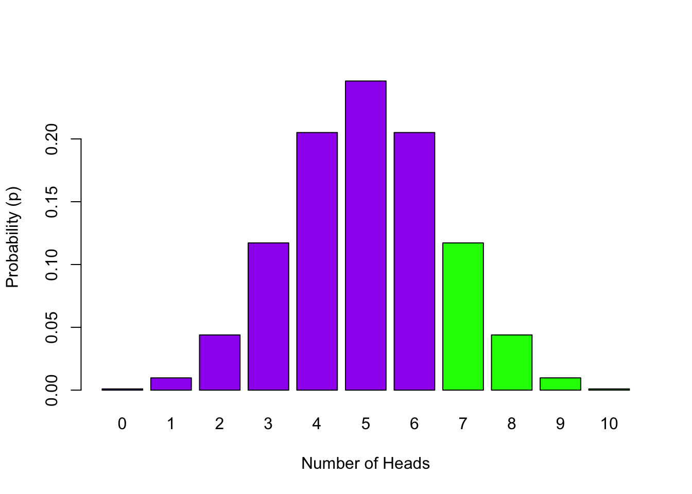
Figure 4.5: Probability Distribution of Number of Heads in 10 Flips with the probability of 7 or more Heads highlighted in green - lower.tail = FALSE
The most confusing part for people we find is the concept of lower.tail. If you look at a distribution, say the binomial, you find a lot of the high bars are in the middle of the distribution and the smaller bars are at the far left and right of the distribution. Well the far left and right of the distribution is called the tail of the distribution - they tend to be an extremity of the distribution that taper off like a.....well like a tail. A lot of the time we will talk of left and right tails but the pbinom() function only ever considers data in relation to the left side of the distribution - this is what it calls the lower.tail.
Let's consider lower.tail = TRUE. This is the default, so if you don't state lower.tail = ... then this is what is considered to be what you want. lower.tail = TRUE means all the values to the left of your value including the value you state. So on the binomial distribution if you say give me the probability of 5 heads or less, then you would set lower.tail = TRUE and you would be counting and summing the probability of 0, 1, 2, 3, 4 and 5 heads. You can check this with dbinom(0:5, 10, .5) %>% sum().
However, if you say give me the probability of 7 or more heads, then you need to do lower.tail = FALSE, to consider the right-hand side tail, but also, you need to set the code as pbinom(6, 10, .5, lower.tail = FALSE). Why 6 and not 7? Because the pbinom() function, when lower.tail = FALSE, starts at the value plus one to the value you state; it always considers the value you state as being part of the lower.tail so if you say 6, it includes 6 in the lower.tail and then gives you 7, 8, 9 and 10 as the upper tail. If you said 7 with lower.tail = FALSE, then it would only give you 8, 9 and 10. This is tricky but worth keeping in mind when you are using the pbinom() function. And remember, you can always check it by using dbinom(7:10, 10, .5) %>% sum() and seeing whether it matches pbinom(6, 10, 0.5, lower.tail=FALSE) or pbinom(7, 10, 0.5, lower.tail=FALSE)
Quickfire Questions
Using the format shown above for the
pbinom()function, enter the code that would determine the probability of up to and including 5 heads out of 20 flips, assuming a probability of 0.5:To two decimal places, what is the probability of obtaining more than but not including 50 heads in 100 flips?
-
You are looking to calcuate the probability of 5 or less heads (
x) out of 20 flips (size), with the probability of 'heads' in one trial (prob) remaining the same. Do you need thelower.tailcall here if you are calculating the cumulative probability of the lower tail of the distribution? -
You are looking to calculate the probability of 51 or more heads (
x), out of 100 flips (size), with the probability of 'heads' in one trial (prob) remaining the same (0.5). Do you need thelower.tailcall here if you are calculating the cumulative probability of the upper tail of the distribution? Remember, because you are not looking at thelower.tail, the value of heads that you enter inpbinom()will not be included in the final calculation, e.g. enteringpbinom(3, 100, lower.tail = FALSE)will give you the probability for 4 and above heads. If you were instead looking at thelower.tail, enteringpbinom(3, 100, lower.tail = TRUE)would give you the probability of 3 and below heads.
-
The code for the first one would be:
pbinom(5, 20, 0.5)orpbinom(5, 20, 0.5, lower.tail = TRUE) -
The code for the second one would be:
pbinom(50, 100, 0.5, lower.tail = FALSE), giving an answer of .46. Remember you can confirm this with:dbinom(51:100, 100, 0.5) %>% sum()
4.2.6 qbinom() - The Quantile Function
The qbinom() function is the inverse of the pbinom() function. Whereas with pbinom() you supply an outcome value x and get a tail probability, with qbinom() you supply a tail probability and get the outcome value that (approximately) cuts off that tail probability. Think how you would rephrase the questions above in the pbinom() to ask a qbinom() question. Worth noting though that qbinom() is approximate with a discrete distribution because of the "jumps" in probability between the discrete outcomes (i.e. you can have probability of 2 heads or 3 heads but not 2.5 heads).
Let's see how these two functions are inverses of one another. Below is code for the probability of 49 heads or less in 100 coin flips
p1 <- pbinom(49, 100, .5, lower.tail = TRUE)
p1
## [1] 0.4602054This tells us that the probability is p = 0.4602054. If we now put that probability (stored in p1) into qbinom we get back to where we started. E.g.
qbinom(p1, 100, .5, lower.tail = TRUE)## [1] 49This can be stated as the number of heads required to obtain a probability of 0.4602054 is 0.4602054. So the qbinom() function is useful if you want to know the minimum number of successes (‘heads’) that would be needed to achieve a particular probability. This time the cut-off we specify is not the number of ‘heads’ we want but the probability we want.
For example say we want to know the minimum number of ‘heads’ out of 10 flips that would result in a 5% heads success rate (a probability of .05), we would use the following code.
qbinom(.05, 10, 0.5, lower.tail = TRUE) ## [1] 2Because we are dealing with the lower tail, this is telling us for a lower tail probability of .05, we would expect at most 2 heads in 10 flips. However, it is important to note that for a discrete distribution, this value is not exact. We can see this by...
pbinom(2, 10, .5, lower.tail = TRUE) ## [1] 0.0546875...which is not exactly p = .05 but very close. This is because the data we are working with is a discrete distribution and so qbinom() gives us the closest category to the boundary.
We found a lot of students asking about qbinom() and how it works when you are inputting two different probabilities as the arguments for qbinom(). Let us try and make things clearer.
First, it is useful to remember that it is the inverse of pbinom(): pbinom() gives you a tail probability associated with x, and qbinom() gives you the closest x that cuts off the specified tail probability. If you understand pbinom() then try reversing the question and see if that helps you understand qbinom().
The qbinom() function is set up as qbinom(p, size, prob). First of all, you have used prob in the previous two functions, dbinom() and pbinom(), and it represents the probability of success on a single trial (here it is the probability of 'heads' in one coin flip, prob = .5). Now, prob represents the probability of success in one trial, whereas p represents the tail probability you want to know about. The function gives you the value of x that would yield that probability you asked for. So you give qbinom() a tail probability of p = .05, in 10 flips, when the probability of a success on any one flip is prob = .5. And it tells you the answer is 2, meaning that getting up to 2 flips on 10 trials has a probability of roughly .05.
qbinom() also uses the lower.tail argument and it works in a similar fashion to pbinom().
Quickfire Questions
- Type in the box, the maximum number of heads associated with a tail probability of 10% (.1) in 17 flips:
The answer would be 6 because the code would be:
qbinom(0.1, 17, 0.5, lower.tail = TRUE)
Remember that you want an overall probability of 10% (p = .1), you have 17 flips in each go (size = 17), and the probability of heads on any one flip is .5 (prob = .5). And you want the maximum number for the lower tail, so the lower.tail is TRUE.
Job Done - Activity Complete!
Excellent! We have now recapped some general probability concepts as well as going over the binomial distribution again. We will focus on the normal distribution in the lab but it would help to read the brief section on as part of the PreClass activities.
Always keep in mind that what you are trying to get an understanding of is that every value in a distribution has a probability of existing in that distribution. That probability may be very large, meaning that, for bell-shaped distributions we have looked at, the value is from the middle of the distribution, or that probability might be rather low, meaning it is from the tail, but ultimately every value of a distribution has a probability.
If you have any questions please post them on the available forums or run them by a member of staff. Finally, don't forget to add any useful information to your Portfolio before you leave it too long and forget. Great work!
4.3 PreClass Activity 2
4.3.1 Continuous Data - Brief Recap on The Normal Distribution
This a very short recap on the normal distribution which will help you work through the rest of this chapter if you read it before attempting the rest. In the first PreClass activity, we have seen how we can use a distribution to estimate probabilities and determine cut-off values (these will play an important part in hypothesis testing in later chapters!), but we have looked only at the discrete binomial distribution. Many of the variables we will encounter will be continuous and tend to show a normal distribution (e.g. height, weight, IQ).
Let's say we're interested in the height of the population of Level 2 psychology students, which we estimate to be between 146cm and 194cm. If we plotted this as a continuous, normal distribution, it will look like:

Figure 4.6: The Normal Distribution of height in Level 2 Psychology students (black line). Green line represents the mean. Blue line represent 1 Standard Deviation from the mean. Yellow line represents 2 Standard Deviation from the mean. Red line represents 3 Standard Deviation from the mean.
The figure shows the hypothetical probability density of heights ranging from 146cm to 194cm in the population of level 2 psychology students (black curve). This data is normally distributed and has the following properties:
4.3.2 Properties of the Normal distribution:
1. The distribution is defined by its mean and standard deviation: The mean (\(\mu\)) describes the center, and therefore peak density, of the distribution. This is where the largest number of the people in the population will be in terms of height. The standard deviation (\(\sigma\)) describes how much variation there is from the mean of the distribution - on the figure, the standard deviation is the distance from the mean to the inflection point of the curve (the part where the curve changes from a upside-down bowl shape to a right-side-up bowl shape).
2. Distribution is symmetrical around the mean: The mean lies in the middle of the distribution and divides the area under the curve into two equal sections - so we get the typical bell-shaped curve.
3. Total area under the curve is equal to 1: If we were to add up the probabilities (densities) for every possible height, we would end up with a value of 1.
4. The mean, median and mode are all equal: A good way to check if a given dataset is normally distributed is to calculate each measure of central tendency and see if they are approximately the same (normal distribution) or not (skewed distribution).
5. The curve approaches, but never touches, the x axis: You will never have a probability of 0 for a given x axis value.
6. The normal distribution follows the Empirical Rule: The Empirical Rule states that 99.7% of the data within the normal distribution falls within three standard deviations (\(\pm3\sigma\)) from the mean, 95% falls within two standard deviations (\(\pm2\sigma\)), and 68% falls within one standard deviation (\(\pm\sigma\)).
Job Done - Activity Complete!
We will look at the normal distribution more in the InClass activity but if you have any questions please post them on forums or ask a member of staff. Finally, don't forget to add any useful information to your Portfolio before you leave it too long and forget.
4.4 InClass Activity 1
We are going to continue our study of distributions and probability to help gain an understanding of how we can end up with an inference about a population from a sample. In the preclass activity, we focused a lot on basic probability and binomial distributions. In this activity, we will focus more on the normal distribution; one of the key distributions in Psychology.
The assignment for this chapter is formative and should not be submitted. This of course does not mean that you should not do it. As will all the formative labs, completing them and understanding them, will benefit you when it comes to completing the summative activities. It will be really beneficial to you when it comes to doing the assignment to have run through both the preclass and inclass activities. You may also want to refer to the Lecture series for help. If you are unclear at any stage please do ask; probability is challenging to grasp at first.
Remember to add useful information to you Portfoilio! One of the main reasons we do this is because there is a wealth of research that says the more interactive you are with your learning, the deeper your understanding of the topic will be. This relates to the Craik and Lockhart (1972) levels of processing model you will read about in lectures. Always make notes about what you are learning to really get an understanding of the concepts. And, most importantly, in your own words!
Reference:
4.4.1 Continuous Data and the Normal Distribution
Continuous data can take any precise and specific value on a scale, e.g. 1.1, 1.2, 1.11, 1.111, 1.11111, ... Many of the variables we will encounter in Psychology will:
- be continuous as opposed to discrete.
- tend to show a normal distribution.
- look similar to below - the bell-shaped curve - when plotted.
But can you name any? Take a couple of minutes as a group to think of variables that we might encounter that are normally distributed. We will mention some as we move through the chapters!
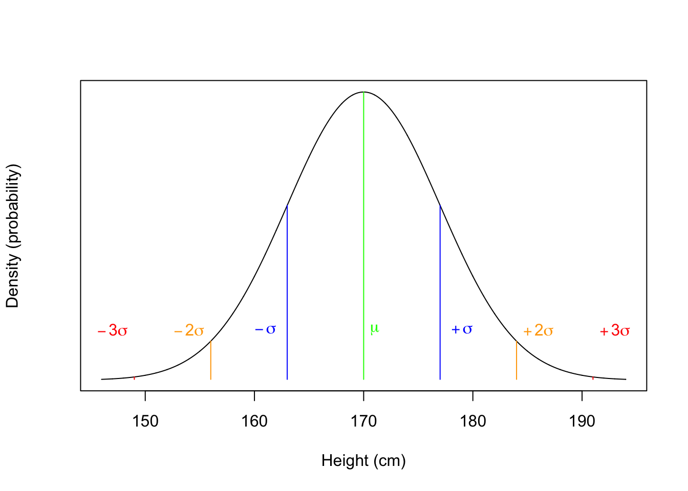
Figure 4.6: The Normal Distribution of height in Level 2 Psychology students (black line). Green line represents the mean. Blue line represent 1 Standard Deviation from the mean. Yellow line represents 2 Standard Deviation from the mean. Red line represents 3 Standard Deviation from the mean.
4.4.2 Estimating from the Normal Distribution
Unlike coin flips, the outcome in the normal distribution is not just 50/50 and as such we won't ask you to create a normal distribution as it is more complicated than the binomial distribution you estimated in the preclass. Instead, just as with the binomial distribution (and other distributions) there are functions that allow us to estimate the normal distribution and to ask questions about the distribution. These are:
dnorm()- the Density function for the normal disributionpnorm()- the Cumulative Probability function for the normal disributionqnorm()- the Quantile function for the normal disribution
You might be thinking those look familiar. They do in fact work in a similar way to their binomial counterparts. If you are unsure about how a function works remember you can call the help on it by typing in the console, for example, ?dnorm or ?dnorm(). The brackets aren't essential for the help.
Quickfire Questions
Type in the box the binomial counterpart to
dnorm()?Type in the box the binomial counterpart to
pnorm()?Type in the box the binomial counterpart to
qnorm()?
The counterpart functions all start with the same letter, d, p, q, it is just the distribution name that changes, binom, norm, t - though we haven't quite come across the t-distribution yet.
-
dbinom()is the binomial equivalent todnorm() -
pbinom()is the binomial equivalent topnorm() -
qbinom()is the binomial equivalent toqnorm()
There is also rnorm() and rbinom() but we will look at them another time.
4.4.3 dnorm() - The Density Function for the Normal Distribution
Using dnorm(), like we did with dbinom, we can plot a normal distribution. This time however we need:
x, a vector of quantiles (in other words, a series of values for the x axis - think of this as the max and min of the distribution we want to plot)- the
meanof our data - and standard deviation
sdof our data.
We will use IQ as an example. There is actually some disagreement of whether or not IQ is continuous data and to some degree it will depend on the measurement you use. IQ however is definitely normally distributed and we will assume it is continuous for the purposes of this demonstration. Many Psychologists are interested in studying IQ, perhaps in terms of heritability, or interested in controlling for IQ in their own studies to rule out any effect (e.g. clinical and autism studies).
4.4.3.1 Task 1: Standard Deviations and IQ Score Distribution
- Copy the below code into a new script and run it. Remember that you will need to call
tidyverseto your library first. e.g.library("tidyverse").
This code creates the below plot showing a normal distribution of IQ scores (M = 100, SD = 15) ranging from 40 to 160. These are values considered typical for the general population.
- First we set up our range of IQ values from 40 to 160
- Then we plot the distribution of IQ_data, where we have M = 100 and SD = 15
IQ_data <- tibble(IQ_range = c(40, 160))

ggplot(IQ_data, aes(IQ_range)) +
  stat_function(fun = dnorm, args = list(mean = 100, sd = 15)) +
  labs(x = "IQ Score", y = "probability") +
  theme_classic()
Figure 4.7: Distribution of IQ scores with mean = 100, sd = 15
- Which part of the code do you need to change to alter the SD of your plot?
- Now copy and edit the above code to plot a distribution with
mean = 100andsd = 10, and visually compare the two plots.
Group Discussion Point
What does changing the standard deviation (sd) do to the shape of the distribution? Spend a few minutes changing the code to various values and running it, and discussing with your group to answer the following questions:
What happens to the shape of the distribution if you change the
sdfrom 10 to 20?What happens to the shape of the distribution if you change the
sdfrom 10 to 5?What does a small or large standard deviation in your sample tell you about the data you have collected?
- Changing the SD from 10 to 20 means a larger standard deviation so you will have a wider distribution.
- Changing the SD from 10 to 5 means a smaller standard deviation so you will have a narrower distribution.
- Smaller SD results in a narrower distribution meaning that the data is less spread out; larger SD results in a wider distribution meaning the data is more spread out.
A note on the Standard Deviation:
You will know from your lectures that you can estimate data in two ways: point-estimates and spread estimates. The mean is a point-estimate and condenses all your data down into one data point - it tells you the average value of all your data but tells you nothing about how spread out the data is. The standard deviation however is a spread estimate and gives you an estimate of how spread out your data is from the mean - it is a measure of the standard deviation from the mean.
So imagine we are looking at IQ scores and you test 100 people and get a mean of 100 and an SD of 5. This means that the vast majority of your sample will have an IQ around 100 - probably most will fall within 1 SD of the mean, meaning that most of your participants will have an IQ of between 95 and 105.
Now if you test again and find a mean of 100 and an SD of 20, this means your data is much more spread out. If you take the 1 SD approach again then most of your participants will have an IQ of between 80 and 120.
So one sample has a very tight range of IQs and the other sample has a very wide range of IQs. All in, from the point-estimate and spread estimate of your data you can tell the shape of your sample distribution.
So far so good! But in the above example we told dnorm() the values at the limit of our range and it did the rest; we said give us a range of 40 to 160 IQ scores. However, we could plot it another way by telling dnorm() the sequence, or range, of values we want and how much precision we want between them.
4.4.3.2 Task 2: Changing Range and Step Size of The Normal Distribution
- Copy the code below in to your script and run it. Here we plot the standard Normal Distribution from -4 to 4 in steps of 0.01. We have also stated a mean of 0 and an sd of 1.
ND_data <- tibble(ND_range = seq(-4, 4, 0.01))
ggplot(ND_data, aes(ND_range)) +
  stat_function(fun = dnorm, args = list(mean = 0, sd = 1)) +
  labs(x = "SD units", y = "probability", title = "The Normal Distribution") +
  theme_classic()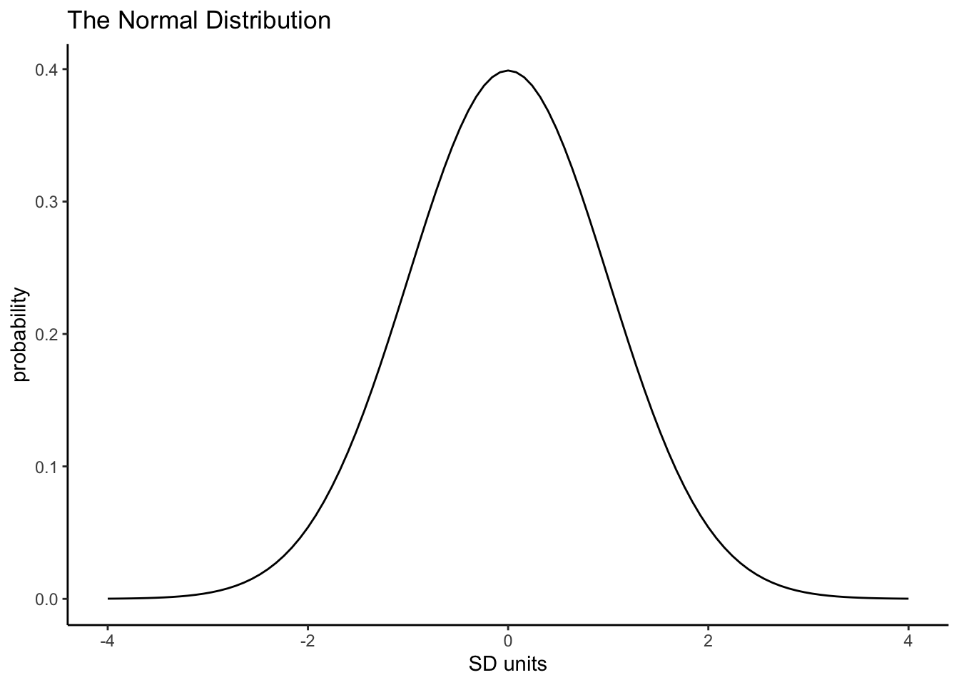
Figure 4.8: The Normal Distribution with Mean = 0 and SD = 1
Quickfire Questions
- Fill in the box to show what you would type to create a tibble containing a column called
ND_rangethat has values ranging from-10to10in steps of.05:
ND_data <-
Now that you know what to change, try plotting a normal distribution with the following attributes:
range of -10 to 10 in steps of 0.05,
a mean of 0,
and a standard deviation of 1.
Compare your new plot the the original one we created. What change is there in the distribution?
To change the distribution you would write: ND_data <- tibble(ND_range = seq(-10, 10, 0.05))
However, when comparing the plots, whilst the plot itself may look thinner, the distribution has not changed. The change in appearance is due to the range of sd values which have been extended from -4 and 4 to -10 and 10. The density of values within those values has not changed however and you will see, more clearly in the second plot, that values beyond -3 and 3 are very unlikely.
Remember, every value has a probability on a distribution and we have been able to use the dnorm() function to get a visual representation of how the probability of values change in the normal distribution. Some values are very probable. Some values are very unpprobable. This is a key concept when it comes to thinking about significant differences later in this series.
However, as you know, there is one important difference between continuous and discrete probability distributions - the number of possible outcomes. With discrete probability distributions there are usually a finite number of outcomes over which you take a probability. For instance, with 5 coin flips, there are 5 possible outcomes for the number of heads: 0, 1, 2, 3, 4, 5. And because the binomial distribution has exact and finite outcomes, we can use dbinom() to get the exact probability for each outcome.
In contrast, with a truly continuous variable, the number of possible outcomes are infinite, because you not only have 0.01 but also .0000001 and .00000000001 to arbitrary levels of precision. So rather than asking for the probability of a single value, we ask the probability for a range of values, which is equal to the area under the curve (the black line in the plots above) for that range of values.
As such, we will leave dnorm() for now and move onto looking at establishing the probability of a range of values using the Cumulative Probability function
4.4.4 pnorm() - The Cumulative Probability function
Just as dnorm() works like dbinom(), pnorm() works just like pbinom(). So, pnorm(), given the mean and sd of our data, returns the cumulative density function (cumulative probability) that a given probability (p) lies at a specified cut-off point and below, unless of course lower.tail = FALSE is specified in which case it is from the cut-off point and above.
OK, in English that people can understand, that means the pnorm() function tells you the probability of obtaining a given value or lower if you set lower.tail = TRUE. Contrastingly, pnorm() function tells you the probability of obtaining a given value or higher if you set lower.tail = FALSE.
We will use height to give a concrete example. Say that we test a sample of students (M = 170cm, SD = 7) and we we want to calculate the probability that a given student is 150cm or shorter we would do the following:
- Remember,
lower.tail = TRUEmeans lower than and including the value of X TRUEis the default so we don't actually need to declare it
pnorm(150, 170, 7, lower.tail = TRUE)This tells us that finding the probability of someone 150cm or shorter in our class is about p = 0.0021374. Stated differently, we would expect the proportion of students to be 150cm or shorter to be 0.21% (You can convert probability to proportion by multiplying the probability by 100). This is a very small probability and suggests that it is pretty unlikely to find someone shorter than 150cm in our class. This is mainly because of how small the standard deviation of our distribution is. Think back to what we said earlier about narrow standard deviations round the mean!
Another example might be, what would be the probability of a given student being 195 cm or taller? To do that, you would set the following code:
pnorm(195, 170, 7, lower.tail = FALSE)This tells us that finding the probability of someone 150cm or shorter in our class is about p = 0.9998225. Or 99.98%. So again, really unlikely.
Did you notice something different about the cut-off for this example and from when using the dbinom() function and looking above a cut-off? Why might that be? We will discuss in a second but first a quick task.
4.4.4.1 Task 3: Calculating Cumulative Probability of Height
- Edit the
pnorm()code above to calculate the probability that a given student is 190cm or taller.
To three decimal places, as in Task 3, what is the probability of a student being 190cm or taller in this class?
The answer is .002. See the solution code at the end of the chapter.
The key thing is that there is a difference in where you need to specify the cut-off point in the pbinom() (discussed in the preclass activity) and pnorm() functions for values above x, i.e. when lower.tail = FALSE.
If you had discrete data, say the number of coin flips that result in heads, and wanted to calculate the probability above x, you would apply pbinom() and have to specify your cut-off point as x-1 to include x in your calculation. For example, to calculate the probability of 4 or more 'heads' occuring in 10 coin flips, you would specify pbinom(3, 10, 0.5, lower.tail = FALSE) as lower.tail includes the value you state.
For continuous data, however, such as height, you would be applying pnorm() and therefore can specify your cut-off point simply as x. In the above example, for the cut-off point of 190, a mean of 170 and standard deviation of 7, you can write pnorm(190, 170, 7, lower.tail = FALSE). The way to think about this is that setting x as 189 on a continuous scale, when you only want all values greater than 190, would also include all the possible values between 189 and 190. Setting x at 190 starts it at 190.0000000...001.
This is a tricky difference between pbinom() and pnorm() to recall easily, so best include this explanation point in your portfolio to help you carry out the correct analyses in the future!
4.4.4.2 Task 4: Using Figures to Calculate Cumulative Probability
Have a look at the distribution below:
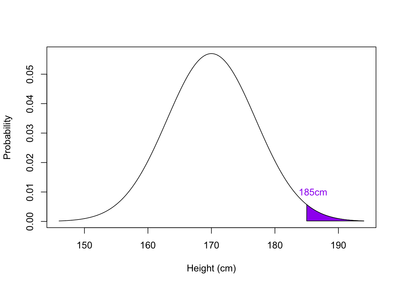
Figure 4.9: The Normal Distribution of Height with the probability of people of 185cm highlighted in purple, with a mean = 170cm and SD = 7
- Using the information in the figure, and the mean and SD as above, calculate the probability associated with the shaded area.
You already have your mean and standard deviations to input in pnorm(), look at the shaded area to obtain your cut-off point. What should the lower.tail call be set to according to the shaded area?
Quickfire Question
To three decimal places, what is the cumulative probability of the shaded area in Task 4?
The answer should be p = .016. See the solution code at the end of the chapter for the correct code.
Remember, lower.tail is set to FALSE as you want the area to the right.
So pnorm() is great for telling us the probability of obtaining a specific value or greater on a distribution, given the mean and standard deviation of the distribution. The significance of this will come clearer in the coming chapters but this is a key point to have in mind as we progress through our understanding of analyses. We will leave it there for now and look at the last function of the normal distribution.
4.4.5 qnorm() - The Quantile Function
Using qnorm() we can do the inverse of pnorm(), and instead of finding out the cumulative probability from a given set of values (or to a cut-off value), we can find a cut-off value given a desired probability. For example, we can use the qnorm() function to ask what is the maximum IQ a person would have if they were in the bottom 10% of the above IQ distribution (M = 100 & SD = 15)?
- Note: We first need to convert 10% to a probability by dividing by 100
- 10% = 10 / 100 = 0.1.
qnorm(0.1, 100, 15) So anyone with an IQ of 80.8 or lower would be in the bottom 10% of the distribution. Or to rephrase that, a person in the bottom 10% of the distribution would have a max IQ value of 80.8.
To recap, we have calculated the inverse cumulative density function (or inverse of the cumulative probability) of the lower tail of the distribution, with a cut-off of a probability of 0.1 (10%), illustrated in purple below:
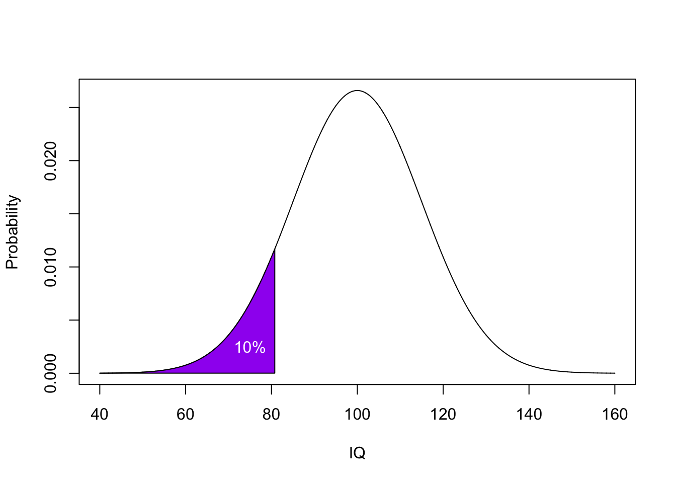
Figure 4.10: The Normal Distribution of Height with the bottom 10% of heights highlighted in purple
Again, in English that people can understand, that means the qnorm() function tells you the maximum value a person can have to maintain a given probability if you set lower.tail = TRUE. Contrastingly, pnorm() function tells you the the minimum value a person can have to maintain a given probability if you set lower.tail = FALSE.
4.4.5.1 Task 5: Using pnorm() and qnorm() to find probability and cut-off values
Calculate the lowest IQ score a student must have to be in the top 5% of the above distribution.
More challenging: Using the appropriate normal distribution function, calculate the probability that a given student will have an IQ between 105 and 110, on a normal distribution of mean = 100, sd = 15.
Part 1: Remember to include the lower.tail call if required! If you are unsure, visualise what you are trying to find (i.e. the lowest IQ score you can have to be in top 5%) by sketching it out on a normal distribution curve. It may help to reverse the question to sound more like the previous example.
Part 2: For the second part, each function, not necessarily qnorm(), gives one value, so you are looking to do a separate calculation for each IQ. Then you have to combine these two values, but are you summing or subtracting them? Is it more or less likely for students to have an IQ that falls between this range than above or below a cut-off? Again try sketching out what you are trying to achieve.
Quickfire Questions
To one decimal place, enter your answer for Task 5 part 1: What is the lowest IQ score a student must have to be in the top 5% of the distribution?
To two decimal places, enter your answer for Task 5 part 2: What is the probability that a student will have an IQ between 105 and 110, on a normal distribution of mean = 100, sd = 15?
-
The question can be rephrased as what value would give you 95% of the distribution - and the answer would be 124.7. See the solution code for Task 5 Question 1 at the end of the chapter.
-
You could use
pnorm()to establish the probability of an IQ of 110. And you could usepnorm()again to establish the probability of an IQ of 105. The answer is the difference between these two probabilities and should be p = .12. See the solution code for Task 5 Question 2 at the end of the chapter.
Job Done - Activity Complete!
You have now recapped probability and the binomial and normal distributions. You should now be ready to complete the Homework Assignment for this lab. The assignment for this Lab is FORMATIVE and is NOT to be submitted and will NOT count towards the overall grade for this module. However you are strongly encouraged to do the assignment as it will continue to boost your skills which you will need in future assignments. If you have any questions, please post them on the available forums for discussion. Finally, don't forget to add any useful information to your Portfolio before you leave it too long and forget.
Excellent work! You are Probably an expert! Now go try the assignment!
4.5 InClass Activity 2 (Additional)
In the preclass activity, we focused a lot on basic probability and binomial distributions. If you have followed it, and understood it correctly, you should be able to have a go at the following scenario to help deepen your understanding of the binomial distribution. Have a go and see how you get on. Solutions are at the end of the chapter.
4.5.1 Return of the Binomial {Ch4InClassQueBinomial}
You design a psychology experiment where you are interested in how quickly people spot faces. Using a standard task you show images of faces, houses, and noise patterns, and ask participants to respond to each image by saying 'face' or 'not face'. You set the experiment so that, across the whole experiment, the number of images per stimuli type are evenly split (1/3 per type) but they are not necessarily evenly split in any one block. Each block contains 60 trials.
To test your experiment you run 1 block of your experiment and get concerned that you only saw 10 face images. As this is quite a low number out of a total of 60 you think something might be wrong. You decide to create a probability distribution for a given block of your experiment to test the likelihood of seeing a face (coded as 1) versus not seeing a face (coded as 0).
You start off with the code below but it is incomplete.
blocks_5k <- replicate(n = NULL,
                       sample(0:1,
                              size = NULL,
                              replace = NULL,
                              c(2/3,1/3)) %>%
sum())- Copy the code to a script and replace the
NULLswith the correct value and statement to establish how many different numbers of faces you might see in 1 block of 60 trials, over 5000 replications. Answering the following questions to help you out:
Quickfire Questions
The
nNULL relates to:The
sizeNULL relates to:replaceshould be set to:
-
replicateis how many times you want to run the sample, n = 5000. Monte Carlo replications are their official name. -
The number of trials is the
size, 60. -
And in order for the code to work, and to not run out of options, you need to set
replaceas TRUE.
You saw a very similar code in the preclass so be sure to have had a look there. The solution code is shown at the end of the chapter
Note that the values in the prob argument (i.e. c(2/3, 1/3) ) set probabilities for the two outcomes specified in the first argument (0, 1). So, we are setting a 2/3 probability of 0 (no face), and a 1/3 probability of 1 (face). Why? Remember that in this instance you have three different stimuli (face, house and noise) and therefore we have a greater chance of not seeing a face in the experiment (i.e. you see a house or noise) than seeing a face in the experiment. You need to remember when using sample (?sample) to set the probability appropriately or you will end up with an incorrect calculation.
- If you completed the above task correctly, your
blocks_5kcode has created 5000 values where each value represents the number of faces you 'saw' in each individual replication (i.e. block) of 60 trials - like the number of heads you saw in 10 flips. If your code has worked, then running the chunk below should produce a probability distribution of your data. Run it and see. If not, something has gone wrong in your code above; debug or compare you code to the solution at the end of the chapter.
data5k <- tibble(faces_per_block = blocks_5k) %>%
  count(faces_per_block) %>%
  mutate(p = n / 5000)
ggplot(data5k, aes(faces_per_block, p)) +
  geom_col() +
  theme_light()
If you view data5k, you will now see three columns:
faces_per_blocktells you all the number of face trials seen in a block of 60 trials. Note that it does not run from 0 to 60.ntells you the number of blocks in which the corresponding number of face trials appeared, e.g. in 228 blocks there were 15 face trials. (Remember this is sampled data so your values may be different!).ptells you the probability of the corresponding number offaces_per_block.
From your data5k tibble, what was the probability of seeing only 10 faces in a block? Ours was 0.002 but remember that we are using a limited number of replications here so our numbers will vary from yours. To find this value you can use View() or glimpse() on data5k.
Group Discussion Point
Discuss in your groups the following questions:
If the probability of seeing only 10 faces was approximately p = 0.002, what does that say about whether our experiment is coded correctly or not?
We only have data for 28 potential different number of face trials within a block. Why does this value not stretch from 0 to 60, or at least have more potential values than 28?
On the first point, it says that the probability of having a block with only 10 faces is pretty unlikely - it has only a small probability. However, it is still possible. Does that say there is an error in your code? Not necessarily as it is possible you just happened to get a block with only 10 faces. Despite it being a low probability it is not impossible. What it might say, however, is that if this is something that concerns you, this potentially low number of faces in a block, then you need to think about the overall design of your experiment and consider having an equal weighting of stimuli in each block.
On the second point, you need to think about the width of the distribution. The probability of a face is 1/3 or p = .33. If there are 60 trials per block then that works out, on average, at approx 20 faces per block . The further you move away from that average, 20, the less probable it is to see that number of faces. E.g. 10 faces had a very low probability as will 30 faces. 40 faces will have almost no probability whatsoever. In only 5000 trials not all values will be represented.
Quickfire Questions
Using the appropriate
binom()function, to three decimal places, type in the actual probability of exactly 10 faces in 60 trials:Using the appropriate
binom()function, to three decimal places, type in the actual probability of seeing more than, but not including, 25 faces in a block of 60 trials?Using the appropriate
binom()function, enter the number of faces needed in a block of 60 trials that would cut off a lower tail probability of .05.
-
You are looking for the probability of one specific value of faces appearing, i.e. 10 faces in a total of 60 trials. You are not looking for the cumulative probability or a range of values. What does this tell you about the apporpriate
binom()function you require? Also, in thesamplefunction, we created a vector of probability dependent on the appearance of both faces and other stimuli. However, for thebinom()function, you need to include only the probability of faces appearing - \(\frac{1}{3}\). -
You are looking for the cumulative probability for seeing more than but not including 25 faces in a block of 60 trials. What does this tell you about the apporpriate
binom()function you require? Remember to set an appropriate call forlower.tail! -
The probability level has been provided for you (5% 0r .05). With this you are looking to find the cutoff value for this tail. What does this tell you about the appropriate
binom()function you require? If you are looking for the probability of values at or below this cutoff, islower.tailset to TRUE or FALSE?
-
The answer would be .002 as you require the density,
dbinom(), of 10 faces out of a possible 60 given a probability of 1/3. The appropriate code is as follows:
Code: dbinom(10, 60, 1/3)
-
The answer would be .068 as you require the cumulative probability,
pbinom(), of more than 25 faces out of 60 given a probability of 1/3. As it is more than 25, setting 25 withlower.tailset as FALSE will give you 26 and above (remember this is a binomial distribution, so where you set your cut-off is very important). The appropriate code is as follows:
Code: pbinom(25, 60, 1/3, lower.tail = FALSE)
-
The answer would be 14 using the
qbinom()function based on wanting to maintain 5% probability of faces in 60 trials. The appropriate code is as follows:
Code: qbinom(.05, 60, 1/3)
Job Done - Activity Complete!
Well done on completing this activty! Once you have completed the main body inclass assignment on the Normal Distribution, you should be ready to complete the assignment for this lab. Good luck and remember to refer back to the codes and questions in this lab and the preclass if you get stuck!.
4.6 InClass Activity 3 (Additional)
One thing we looked at in the lecture and in the preclass activity were some rather "basic" ideas about probability using cards. Here is a couple of very quick questions using dice (or die if you prefer) to make sure you understand this.
Have a go and see how you get on. If you don't get the right answers, be sure to post any questions on the available forums for discussions. Finally, don't forget to add any useful information to your Portfolio before you leave it too long and forget.
4.6.1 Back to Basics
Show your answer either as a fraction (e.g. 1/52) or to 3 decimal places (e.g. 0.019).
What is the probability of rolling a 4 on a single roll of a six-sided dice?
What is the probability of rolling a 4, 5 or 6 on a single roll?
What is the probability of rolling a 4 and then a 6 straight after?
Remember:
- Probability is the number of times or ways an event can occur divided by the total number of all possible outcomes.
- When you have two separate events, the probability of them both happening is the joint probability which is calculated by mutliplying all the individual probabilities together.
-
.167 as you have 1 outcome over 6 possibilities - \(\frac{1}{6}\)
-
.5 as you have 3 outcomes over 6 possibilities - \(\frac{3}{6}\)
-
.028 as you have 1 out of 6 on both occasions so the joint probability is used - \(\frac{1}{6} * \frac{1}{6}\). In this instance we do not have to worry about replacement as a dice always has 6 values. Unless of course you were to rub off a value after each roll of the dice but then that would be pretty unusual and you would go through dice pretty quickly, making them rather redundant little square cubes. Probably best we just assumed that didn't happen, we never talk about it again, and we assume replacement in this instance.
Job Done - Activity Complete!
Well done on completing this activity! Once you have completed the main body inclass assignment on the Normal Distribution, you should be ready to complete the assignment for this lab. Good luck and remember to refer back to the codes and questions in this lab and the preclass if you get stuck!.
4.7 Test Yourself
This is a formative assignment meaning that it is purely for you to test your own knowledge, skill development, and learning, and does not count towards an overall grade. However, you are strongly encouraged to do the assignment as it will continue to boost your skills which you will need in future assignments. You will be instructed by the Course Lead on Moodle as to when you should attempt this assignment. Please check the information and schedule on the Level 2 Moodle page.
Lab 4: Formative Probability Assignment!
In order to complete this assignment, you first have to download the assignment .Rmd file which you need to edit - titled GUID_Level2_Semester1Lab4.Rmd. This can be downloaded within a zip file from the link below. Once downloaded and unzipped you should create a new folder that you will use as your working directory; put the .Rmd file in that folder and set your working directory to that folder through the drop-down menus at the top. Download the Assignment .zip file from here.
Now open the assignment .Rmd file within RStudio. You will see there is a code chunk for each of the 10 tasks. Much as you did in the previous assignments, follow the instructions on what to edit in each code chunk. This will often be entering code or a single value and will be based on the skills learnt in the current lab as well as all previous labs.
4.7.1 Today's Topic - Probability
In the lab you recapped and expanded on your understanding of probability, including a number of binom and norm functions as well as some more basic ideas on probability. You will need these skills to complete the following assignment so please make sure you have carried out the PreClass and InClass activities before attempting this formative assignment. Remember to follow the instructions and if you get stuck at any point to questions on the forums.
Before starting let's check
- The .Rmd file is saved into a folder on your computer that you have access to and you have manually set this folder as your working directory. For assessments we ask that you save it with the format GUID_Level2_Semester1_Lab4.Rmd where GUID is replaced with your GUID. Though this is a formative assessment it may be good practice to do the same here.
Note: You should complete the code chunks below by replacing the NULL (except the library chunk where the appropriate code should just be entered). Not all answers require coding. On those that do not require code, you can enter the answer as either code, mathematical notation, or an actual single value. Pay attention to the number of decimal places required.
4.7.2 Load in the Library
There is a good chance that you will need the tidyverse library at some point in this exercise so load it in the code chunk below:
# hint: something to do with library() and tidyverseBasic probability and the binomial distribution questions
Background Information: You are conducting an auditory discrimination experiment in which participants have to listen to a series of sounds and determine whether the sound was human or not. On each trial participants hear one brief sound (100 ms) and must report whether the sound was from a human (coded as 1) or not (coded as 0). The sounds were either: a person, an animal, a vehicle, or a tone, with each type of sound equally likely to appear.
4.7.3 Assignment Task 1
On a single trial, what is the probability that the sound will not be a person? Replace the NULL in the t1 code chunk with either mathematical notation or a single value. If entering a single value, give your answer to two decimal places.
t1 <- NULL4.7.4 Assignment Task 2
Over a sequence of 4 trials, with one trial for each sound, and sampled with replacement, what is the probability of the following sequence of sounds: animal, animal, vehicle, tone? Replace the NULL in the t2 code chunk with either mathematical notation or a single value. If entering a single value, give your answer to three decimal places.
t2 <- NULL4.7.5 Assignment Task 3
Over a sequence of four trials, with one trial for each sound, without replacment, what is the probability of the following sequence of sounds: person, tone, animal, person? Replace the NULL in the t3 code chunk with either mathematical notation or a single value.
t3 <- NULL4.7.6 Assignment Task 4
Replace the NULL below with code, using the appropriate binomial distribution function, to determine the probability of hearing exactly 17 'tone' trials in a sequence of 100 trials. Assume the probability of a tone on any single trial is 1 in 4. Store the output in t4.
t4 <- NULL4.7.7 Assignment Task 5
Replace the NULL below with code using the appropriate binomial distribution function to determine what is the probability of hearing 30 'vehicle' trials or more in a sequence of 100 trials. Assume the probability of a vehicle trial on any one trial is 1 in 4. Store the output in t5.
Hint: do we want the upper or lower tails of the distribution?
t5 <- NULL4.7.8 Assignment Task 6
If a block of our experiment contained 100 trials, enter a line of code to run 10000 replications of one block, summing how many living sounds were heard in each replication. Code 1 for living sounds (person/animal) and 0 for non living sounds (vehicle/tone) and assume the probability of a living sound on any given trial is \(p = .5\).
t6 <- NULLNormal Distribution Questions
Previously, in Lab 2, we looked at an ageing research project investigating differences in visual processing speed between younger (M = 22 years) and older adults (M = 71 years). One check in this experiment, prior to further analysis, is to make sure that older participants do not show signs of mild cognitive impairment (early symptoms of Alzheimer's disease). To do this, we carry out a battery of cognitive tests to screen for such symptoms. One of the tests is the D2 test of attention which is a target cancellation task (i.e. participants cross out all letter d's with two dashes from a line of letters - see Lab 2 for an example). It is designed to test peoples' selective and sustained attention and visual scanning speed. The results of the test give a single score of Concentration Performance for each participant. The key piece of information for this analysis is that the distributions of D2 test scores are typically normally distributed (M = 100, SD = 10).
4.7.9 Assignment Task 7
Replace the NULL below with code using the appropriate function to determine the probability that a given participant will have a D2 score of 90 or lower? Store the output in t7
t7 <- NULL4.7.10 Assignment Task 8
Replace the NULL below with code using the appropriate function to determine the probability that a given participant will have a D2 score of 120 or more? Store the output in t8
t8 <- NULL4.7.11 Assignment Task 9
Replace the NULL below with code using the appropriate function(s) to determine what is the difference in scores that cut off the top 5% and bottom 5% of the distribution? Store the output in t9.
t9 <- NULL4.7.12 Assignment Task 10
Finally, if a participant says to you that they are worried because they have heard that their Concentration Performance was in the bottom 2% of scores on the distribution, what is the maximum D2 score that they can have? Replace the NULL below with a single value to two decimal places. Do not enter code. Store this in t10
t10 <- NULL
Job Done - Activity Complete!
Well done, you are finshed! Now you should go check your answers against the solutions at the end of the chapter. You are looking to check that questions looking for a single value have the same answer as you, and that questions asking for code have the same code as you or give the same answer where alternative variations in the code are allowed (e.g. including lower.tail = TRUE or not including it as it is default). Remember that a single value is not the same as a coded answer and that spelling matters, replicate() is not the same as replicat(). Where there are alternative answers, it means that you could have submitted any one of the options as they should all return the same answer. If you have any questions, please post them on the forums!
Lastly, keep in mind the main point about probability, that we are interested in determining the probability of a given value on a distribution! That is what it is all about and is what we will look at more of in Chapter 5.
4.8 Solutions to Questions
Below you will find the solutions to the questions for the Activities for this chapter. Only look at them after giving the questions a good try and speaking to the tutor about any issues.
4.8.1 InClass Activities
4.8.1.1 InClass Task 1
- First we set up our range of IQ values from 40 to 160
- Then we plot the distribution of IQ_data, where we have M = 100 and SD = 10
library(tidyverse)

IQ_data <- tibble(IQ_range = c(40, 160))

ggplot(IQ_data, aes(IQ_range)) +
  stat_function(fun = dnorm, args = list(mean = 100, sd = 15)) +
  labs(x = "IQ Score", y = "probability") +
  theme_classic()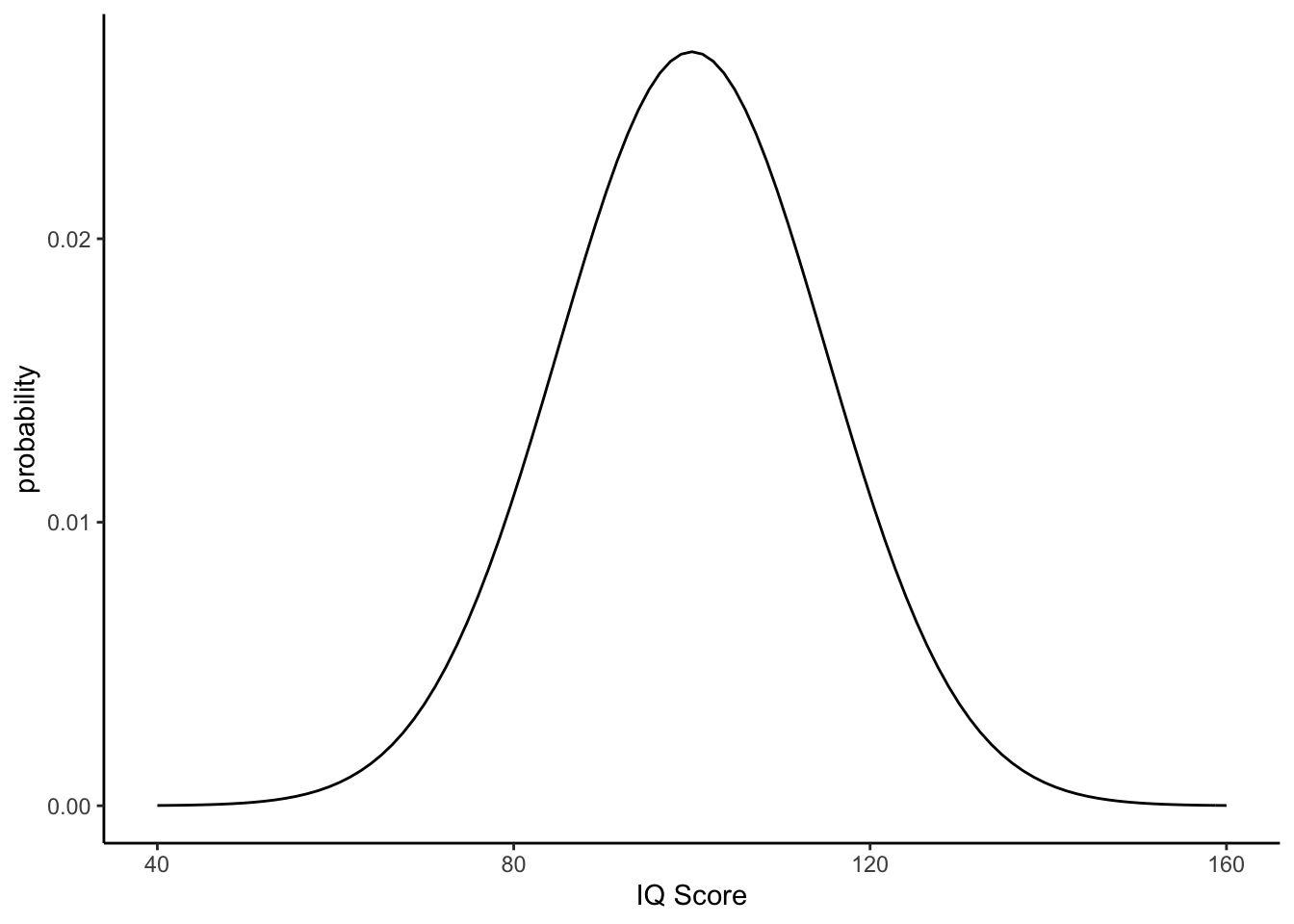
Figure 4.11: Distribution of IQ scores with mean = 100, sd = 10
4.8.1.2 InClass Task 2
ND_data <- tibble(ND_range = seq(-10,10,0.05))

ggplot(ND_data, aes(ND_range)) +
  stat_function(fun = dnorm, args = list(mean = 0, sd = 1)) +
  labs(x = "SD units", y = "probability", title = "The Normal Distribution") +
  theme_classic()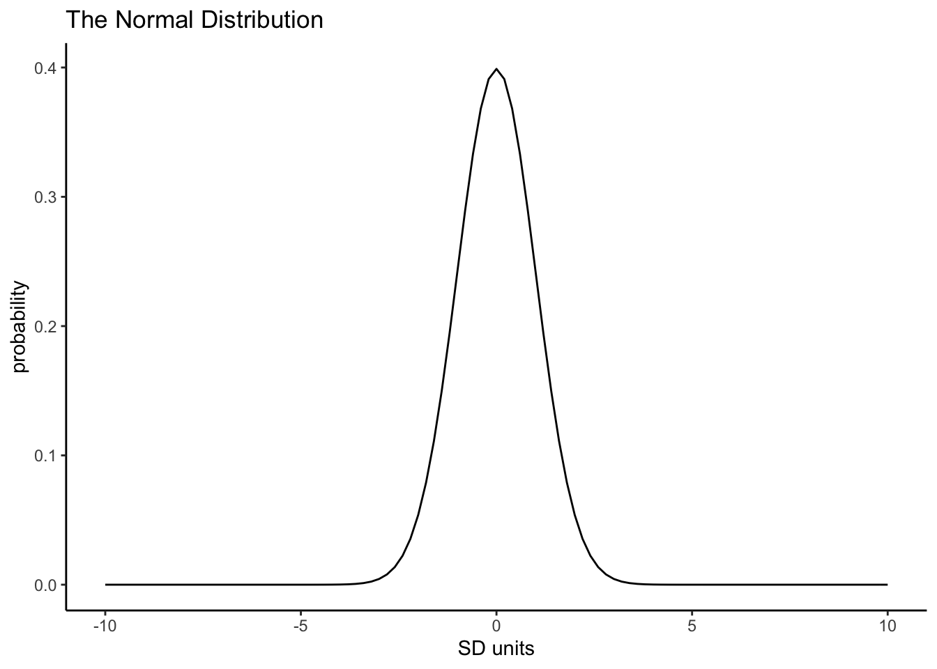
Figure 4.12: Normal Distribution shown on a scale of -10 to 10, with a mean = 0, sd = 1
4.8.1.3 InClass Task 3
- Key thing is to set lower.tail to FALSE to calculate the above area. When using
pnorm()you state the actual cut-off even if usinglower.tail = FALSE. If usingpbinom()you state the cut-off minus one if usinglower.tail = FALSE
pnorm(190, 170, 7, lower.tail = FALSE)## [1] 0.0021373674.8.1.4 InClass Task 4
- The highlighted area is 185cm and above.
- Key thing is to set lower.tail to FALSE to calculate the area from the cut-off and above.
pnorm(185, 170, 7, lower.tail = FALSE)## [1] 0.016062294.8.1.5 InClass Task 5
- Question 1 - the lowest IQ score a student must have to be in the top 5% of the above distribution.
qnorm(0.95, 100, 15, lower.tail = TRUE)## [1] 124.6728- Question 2 - calculate the probability that a given student will have an IQ between 105 and 110, on a normal distribution of mean = 100, sd = 15.
pnorm(105, 100, 15, lower.tail = FALSE) -
  pnorm(110, 100, 15, lower.tail = FALSE)
## [1] 0.11694884.8.2 Return of the Binomial
4.8.2.1 Task 1
blocks_5k <- replicate(n = 5000,
                       sample(0:1,
                              size = 60,
                              replace = TRUE,
c(2/3,1/3)) %>% sum())4.8.3 Test Yourself Activities
4.8.3.2 Assignment Task 1
t1 <- 3/4
t1 <- .75- The probability that the sound will not be a person is 0.75
4.8.3.3 Assignment Task 2
t2 <- (1/4) * (1/4) * (1/4) * (1/4)
t2 <- .004- The probability of that sequence of sounds is 0.004
4.8.3.4 Assignment Task 3
t3 <- (1/4) * (1/3) * (1/2) * (0/1)
t3 <- 0- The probability of that sequence of sounds is 0
- The reason is that there is no replacement and as such the repeat of the
persontrial can't happen.
4.8.3.5 Assignment Task 4
t4 <- dbinom(17, 100, 1/4)- Assuming a probability of a tone on a given trial is 1 in 4, the probability of hearing 17 'tone' trials in a sequence of 100 trials is 0.0165156
4.8.3.6 Assignment Task 5
- This could have been answered using either
pbinom()ordbinom(). The trick is to remember where to set the cut-off depending on the function used.
t5 <- pbinom(29, 100, 1/4, lower.tail = FALSE)
t5 <- dbinom(30:100, 100, 1/4) %>% sum()- In this scenario, the probability of hearing 30 'vehicle' trials or more in a sequence of 100 trials is 0.149541
4.8.3.7 Assignment Task 6
- The appropriate code would be:
t6 <- replicate(10000, sample(0:1, 100, TRUE, c(.5,.5)) %>% sum())If you were to look at your output you would see something like the following. Remember your numbers will vary from ours due to random sampling. Here we are only showing the first 10 values of 10000
## int [1:10000] 44 54 47 52 54 45 54 48 48 55 ...4.8.3.8 Assignment Task 7
t7 <- pnorm(90, 100, 10, lower.tail = TRUE)- The probability of a given participant having a D2 score of 90 or lower is 0.1586553
4.8.3.9 Assignment Task 8
t8 <- pnorm(120, 100, 10, lower.tail = FALSE)- The probability that a given participant will have a D2 score of 120 or more is 0.0227501
4.8.3.10 Assignment Task 9
t9 <- qnorm(.95, 100, 10) - qnorm(.05, 100, 10)- The difference in scores that cut off the top and bottom 5% of the distribution is 32.8970725
4.8.3.11 Assignment Task 10
t10 <- 79.46- The maximum D2 score that they can have in this situation is 79.46
Chapter Complete!