Lab 5 Permutation Tests - A Skill Set

5.1 Overview

To many, a lot of statistics must seem a bit like blind faith as it deals with estimating quantities, values and differences we haven’t observed (or can’t observe), e.g. the mean of a whole population. As such, we have to know if we can trust our statistical analyses and methods for making estimations and inferences because we rarely get a chance to compare the estimated values (e.g. from a sample) to the true values (e.g. from the population) to see if they match up. One way to test a procedure, and in turn learn about statistics, is through data simulation. In simulations, we create a population and then draw samples and run tests on the data, i.e. on this known population. By running lots of simulations we can test our procedures and make sure they are acting as we expect them to. This approach is known as a Monte Carlo simulation, named after the city famous for the many games of chance that are played there.

You can go read up on the Monte Carlo approach if you like. It can, however, get quite indepth, as having a brief glance at the wikipedia entry on it highlights. The main thing to keep in mind is that the method involves creating a population and continually taking samples from that population in order to make an inference. This is what we will show you in this chapter. Data simulation and “creating” your own datasets, to see how tests work, is a great way to understand statistics.

Something else to keep in mind, when doing this chapter, is how easy it really is to find a significant result if even randomly created data can give a significant result. This may help dispell any notion that there is something inherently important about a significant result, in itself.

In this chapter, you will perform your first hypothesis test using a procedure known as a permutation test. We will help you learn how to do this through building and running data simulation procedures. So overall the aims of this chapter are to:

1. Learn how to write code to simulate data
2. Learn about hypothesis testing for significant differences through a permutation test

Now you may be thinking simulating data sounds very much like making fake data which you know is one of the Questionable Research Practices (QRP) that has lead to issues in the past. Let’s be clear, faking data for the purpose of finding an enviable result and publishing it (or even just telling people about it as though it is a real result) is very wrong. Never ever do this! It has unfortunately happened in the past and likely still happens. You can read more about the consequences and prevalences of faking data in John, Loewenstein & Prelec (2012) or in Chapter 5 of Chris Chambers’ excellent book, “The seven deadly sins of psychology: a manifesto for reforming the culture of scientific practice,” under the sin of Corruptability. There are three copies of this book in the University of Glasgow library (and Phil says you can borrow his if you promise to give it on to someone else after you have finished it!)

Simulating data however is not a QRP as the intent is to test your analytical methods and to test statistical theory. You simulate data to see how certain statistical tests wourk under different conditions (e.g. big or small difference between conditions). Alternatively, you simulate data to test your analysis code is working whilst you collect data - running an experiment takes time and so as you are gathering data, you can be using simulated data in the same shape as your eventual data to test your analysis code. Then when you have your actual data you just swap the simulated data for the real data. This is a great thing to do as it allows you to check ahead of evening running the experiment that your analysis will work and that you have not forgotten to collect some important piece of information - think of Registered Reports as discussed in Munafo et al., (2019). Lastly, maybe you want to simulate data to practice hand calculations to learn about tests. Even learning about a mean requires data so you can simulate data numerous times for yourself to practice hand calculating a mean.

As you can see there is a lot of important and useful reasons to learn about simulating data. And that it is very different from faking data. Simulating data is a very useful tool in a researcher’s toolbox. Faking data is very bad practice, often illegal, and you should never do it or feel pressured by anyone else to fake data. If you are ever in this situation please feel free to reach out to the authors of this book.

In order to complete this chapter you will require the following skills, which we will teach you today:

• Skill 1: Generating random numbers with base::rnorm()
• Skill 2: Permuting values with base::sample()
  
• Skill 3: Creating a “tibble” (a type of data table) using tibble::tibble()
• Skill 4: Computing and extracting a difference in group means using dplyr::pull() and purrr::pluck()
• Skill 5: Creating your own custom functions using base::function()
• Skill 6: Repeating operations using base::replicate()

5.2 PreClass Activity

We will now take each skill in turn. Be sure to try them all out. It looks a lot of reading but it is mainly just showing you the output of the functions so you can see you are using them correctly. The key thing is to try them yourselves and don’t be scared to change things to see what might happen if you do it slightly differently. We will also ask a couple of questions along the way to make sure you are understanding the skills.

The trick with this chapter is to be always thinking about the overarching aim of: 1) learning about simulating data, and 2) learning about hypothesis testing. This PreClass activity is setting up the skills to simulate data. We will get to the actual use of it in the InClass activity.

5.2.1 Skill 1: Generating Random Numbers

The first step in any simulated dataset is getting some numbers. We can use the base::rnorm() function to generates values from the normal distribution which we saw in Chapter 4. It is related to the dnorm(), pnorm() and qnorm() functions we have already seen. Where as those functions ask questions of the normal distribution, the rnorm() generates values based on the distribution and takes the following arguments:

• n: the number of observations to generate
• mean: the mean of the distribution (default 0)
• sd : the standard deviation of the distribution (default 1)

For example, to generate 10 or even 50 random numbers from a standard normal distribution (M = 0, SD = 1), you would use rnorm(10, 0, 1) or rnorm(50, 0, 1) respectively.

• Type rnorm(50, 0, 1) into your console and see what happens. Use the below example for rnorm(10, 0, 1) to help you.
  
• Try increasing n to 1000.

rnorm(10, 0, 1)

##  [1]  0.4718362 -1.2382692 -1.2042214 -0.2418053 -0.6838115  0.7842449
##  [7] -0.9419668  1.3458579  0.9236536  1.9262364

Quickfire Question

• If you enter rnorm(50, 0, 1) again you will get different numbers. Why? I have made a mistake The numbers are random R has made a mistake Phil has made a mistake

So far so good. One thing worth pointing out is that the default arguments to rnorm() for mean and sd are mean = 0 and sd = 1. What that means in practice is that you don’t have to write rnorm(10, 0, 1) all the time if you just want to use those default mean and sd values. Instead you could just write rnorm(10) and it would work just as well giving you ten values from a normal distribution of mean = 0 and sd = 1. But let’s say you want to change the mean or sd, then you would need to pass (and change) the mean and sd arguments to the function as shown below.

rnorm(n = 10, mean = 1, sd = .5)

• Try changing the mean and sd values a couple of times and see what happens. You get different numbers again that will be around the mean you set! Set a mean of 10, then a mean of 100, to test this.

Great. We can now generate numbers. But finally, for this Skill, say you wanted to create a vector with two sets of 50 random numbers from two separate samples: one set of 50 with a mean of 75 (sd = 1) and the other with a mean of 90 (sd = 1) - almost like creating two groups. In this case you would concatenate (i.e. link) numbers created from two separate rnorm() calls together into a single vector using the c() function from base R.

For example, you would use:

random_numbers <- c(rnorm(50, 75),
                    rnorm(50, 90))

Quickfire Questions

• In the above example code, what is the standard deviation of the two samples you have created? 50 75 90 1

What is the default sd of the function?

Both populations would have an sd of 1, because that is the default. Remember if there is a default value to an argument then you don’t have to state it in the code.

Remember you can also easily change the sd value of each rnorm() by just adding sd = … to each function. They can have the same sd or different sds. Try it out!

One useful thing though, as mistakes happen, it is always good to check that your new vector of numbers has the right number of data points in it - i.e. the total of the two samples; a sanity check if you will. The new vector random_numbers should have 100 elements. You could verify this using the length() function:

length(random_numbers)

Which tells us that we have generated 100 numbers just as expected! Awesome. Check us out - already mastered generating random numbers!

Skill 1 out of 6 Complete!

5.2.2 Skill 2: Permuting Values

Another skill that is useful to be able to do is to generate permutations of values. Say for example you have already the values collected, with certain numbers atttributed to group A and certain numbers attributed to group B. Permutating those values allows you to change who was in what group and allows you to ask if there was some important difference between the groups based on their original values.

A permutation is just a different ordering of the same values. For example, the numbers 1, 2, 3 can be permuted into the following 6 sequences:

• 1, 2, 3
• 1, 3, 2
• 2, 1, 3
• 2, 3, 1
• 3, 1, 2
• 3, 2, 1

The more values you have, the more permutations of the order you have. The number of permutations can be calculated by, for example, 3 x 2 x 1 = 6, where 3 is the number of values you have. Or through code: factorial(3) = 6. This assumes that each value is used once in the sequence and that each value never changes, i.e. 1234 cannot suddenly become 1235.

We can create random permutations of a vector using the sample() function. Let’s use one of R’s built in vectors: letters.

• Type letters into the console, as below, and press RETURN/ENTER. You will see it contains all the lowercase letters of the English alphabet. Now, I bet you are wondering what LETTERS does, right?

letters

##  [1] "a" "b" "c" "d" "e" "f" "g" "h" "i" "j" "k" "l" "m" "n" "o" "p" "q" "r" "s"
## [20] "t" "u" "v" "w" "x" "y" "z"

We can use the base::sample() function with letters to put the letters into a random order:

• Run the below line. Run it again. And again. What do you notice? And why is our output different from yours? (The answer is below)

sample(letters)

##  [1] "c" "u" "d" "f" "i" "e" "a" "w" "p" "x" "k" "t" "q" "h" "s" "y" "v" "z" "l"
## [20] "o" "j" "n" "r" "m" "g" "b"

Quickfire Questions

• If month.name contains the names of the twelve months of the year, how many possible permutations are there of sample(month.name)? 1 12 144 479001600

Each time you run sample(letters) it will give you another random permutation of the sequence. That is what sample() does - creates a random permutation of the values you give it. Try repeating this command many times in the console. Because there are so many possible sequences, it is very unlikely that you will ever see the same sequence twice!

An interesting thing about sample() is that sample(c(1,2,3,4)) is the same as sample(4). And to recap, there would be 24 different permutations based on factorial(4), meaning that each time you type sample(4) you are getting one of those 24 different orders. So what would factorial(12) be?

Top Tip: Remember that you can scroll up through your command history in the console using the up arrow on your keyboard; this way, you don’t ever have to retype a command you’ve already entered.

And thinking about Skill 1 (generate) and Skill 2 (permute) we could always combine these steps with code such as:

random_numbers <- c(rnorm(5, 75),rnorm(5, 90))
random_numbers_perm <- sample(random_numbers)

The first line of code creates the random_numbers - two sets of five.

random_numbers

##  [1] 74.35868 74.17160 75.91439 76.84620 73.71939 89.19206 91.11152 89.41236
##  [9] 90.28996 90.47787

And the second line permutes those numbers into a different order

random_numbers_perm

##  [1] 74.17160 91.11152 90.28996 89.41236 75.91439 89.19206 76.84620 73.71939
##  [9] 90.47787 74.35868

Brilliant! We can now permutate values as well as generate them. The importance of this in hypothesis testing will become clearer as the chapter goes on, but as a teaser, remember that probability is the likelihood of obtaining a specific value in consideration of all possible outcomes.

Skill 2 out of 6 Complete!

5.2.3 Skill 3: Creating Tibbles

Working with tables/tibbles is important because most of the data we want to analyze comes in a table, i.e. tabular form. There are different ways to get tabular data into R for analysis. One common way is to load existing data in from a data file (for example, using readr::read_csv() which you have seen before). But other times, you might want to just type in data directly. You can do this using the tibble::tibble() function - you have seen this function a couple of times already in this book.

Being able to create a tibble of data is a very useful skill when you will want to create some data on the fly just to try certain codes or functions.

5.2.3.1 Entering Data into a Tibble

The tibble() function takes named arguments - this means that the name you give each argument within the tibble function, e.g. Y = rnorm(10) will be the name of the column that appears in the table, i.e. Y. It’s best to see how it works through an example.

The below command creates a new tibble with one column named Y, and the values in that column are the result of a call to rnorm(10): 10 randomly sampled values from a standard normal distribution (mean = 0, sd = 1), as we learnt in Skill 1.

tibble(Y = rnorm(10))

Y
0.6275753
-1.3282050
0.9986710
-1.0552458
1.0973749
1.2884957
-1.0587038
0.8326353
-0.1169799
0.7732466

If, however, we wanted to sample from two different populations for Y, we could combine two calls to rnorm() within the c() function. Again this was in Skill 1, here we are now just storing it in a tibble. See below:

tibble(Y = c(rnorm(5, mean = -10), 
             rnorm(5, mean =  20)))

Y
-9.584343
-11.526960
-9.602943
-9.259919
-10.418807
20.532379
19.869586
19.902063
19.244200
20.431410

Now we have sampled a total of 10 observations - the first 5 come from a group with a mean of -10, and the second 5 come from a group with a mean of 20. Try changing the values in the above example to get an idea of how this works. Maybe even add a third group!

Great. We have combined Skills 1 and 3 to create a tibble of data that we can start to work with. But, of course, it would be good to know which group/condition each data point refers to and so we should add some group names. We can do this using the base::rep() function.

5.2.3.2 Repeating Values to Save Typing

But before finalising our tibble, and adding in the groups, it will help to learn a little about rep(). This function is most useful for automatically repeating conditions/values/data in order to save typing. For instance, if we wanted 20 letter “A”s in a row, we would type:

rep("A", times = 20)

##  [1] "A" "A" "A" "A" "A" "A" "A" "A" "A" "A" "A" "A" "A" "A" "A" "A" "A" "A" "A"
## [20] "A"

The first argument to rep() is the vector containing the information you want repeated, (i.e. the letter A), and the second argument, times, is the number of times to repeat it; in this case 20.

If you wanted to add more information, e.g. if the first argument has more than one element, say groups A and B, it will repeat the entire vector that number of times; A B, A B, A B, … . Note that we enclose “A” and “B” in the c() function, and with quotes, so that it is seen as a single argument or list that we want repeating. The quotes around A and B (i.e. “A”) are saying that these are character data.

rep(c("A", "B"), times = 20)

##  [1] "A" "B" "A" "B" "A" "B" "A" "B" "A" "B" "A" "B" "A" "B" "A" "B" "A" "B" "A"
## [20] "B" "A" "B" "A" "B" "A" "B" "A" "B" "A" "B" "A" "B" "A" "B" "A" "B" "A" "B"
## [39] "A" "B"

Ok that works if we want a series of A B A B etc. But sometimes we want a specific number of As followed by a specific number of Bs; A A A B B B - meaning something like everyone in Grp A and then everyone in Grp B.

We can do this as well! If the times argument has the same number of elements as the vector given for the first argument, it will repeat each element of the first vector as many times as given by the corresponding element in the times vector. In other words, for example, times = c(2, 4) for vector c("A", "B") will give you 2 As followed by 4 Bs.

rep(c("A", "B"), times = c(2, 4))

## [1] "A" "A" "B" "B" "B" "B"

Quickfire Questions

• The best way to learn about this function is to play around with it in the console and see what happens. Answering these questions will help. From the dropdown menus, the correct output of the following function would be:

1. rep(c("A", "B", "C"), times = (2, 3, 1)) - A A A B B C A A B B B C A A B B C C A B C A B C

2. rep(1:5, times = 5:1) - 1 2 3 4 5 1 2 3 4 5 1 2 3 4 5 5 5 5 5 5 4 4 4 4 3 3 3 2 2 1 1 1 1 1 1 2 2 2 2 3 3 3 4 4 5 1 1 1 1 1 1 1 1 5 5 5 5 5 5 5

5.2.3.3 Bringing it Together in a Tibble

Great. Let’s get back to creating our tibble of data. Now we know rep(), we can complete our tibble of simulated data by combining what we’ve learned about generating random numbers (Skill 1) and repeating values (Skill 3). We want our table to look like this:

group	Y
A	-11.435732
A	-9.123214
A	-10.581591
A	-9.892297
A	-9.745320
B	19.710862
B	19.769016
B	20.727771
B	18.677838
B	21.008002

You now know how to create this table. Have a look at the code below and make sure you understand it. We have one column called group where we create As and Bs through rep(), and one column called Y, our data, all in our tibble():

• Note: We have not stated times = in the below code but because of how the rep() function works it knows that the c(5,5) should be read as times = c(5,5). This is not magic. Again it is about defaults and order or arguments. Just like you saw with rnorm() and not having to state mean and sd each time.

tibble(group = rep(c("A", "B"), c(5, 5)),
       Y = c(rnorm(5, mean = -10), rnorm(5, mean =  20)))

• Be sure to play around with the code chunk above to get used to it.
  • Try adding a third group or even a third column? Perhaps you want to give every participant a random age with a mean of 18, and an sd of 1; or even a participant number.

Try row_number() to create participant numbers.

Don’t forget, if you wanted to store your tibble, you would just assign it to a name, such as my_data:

• Note: we are using the row_number() function to give everyone a unique ID.

my_data <- tibble(ID = row_number(1:10), 
                    group = rep(c("A", "B"), c(5, 5)),
                    Y = c(rnorm(5, mean = -10), rnorm(5, mean =  20)),
                    Age = rnorm(10, 18, 1))

which would give a table looking like:

Table 5.1: Simulated data of two groups: Group A (M = -10, SD = 1) and Group B (M = 20, SD = 1). Each participant has been given a unique ID based on row number and a random age

ID	group	Y	Age
1	A	-12.21979	17.33688
2	A	-10.88400	20.75731
3	A	-12.20528	18.35845
4	A	-10.77000	18.63691
5	A	-10.17820	17.87753
6	B	19.00950	16.78803
7	B	19.25667	18.44292
8	B	18.60762	17.86343
9	B	19.89482	18.59709
10	B	19.21873	17.44738

Fabulous! We are really starting to bring these skills together!

Skill 3 out of 6 Complete!

5.2.4 Skill 4: Computing Differences in Group Means

OK so now that we have created some data we want to look at answering questions about that data. For example, the difference between two groups. Thinking back to Chapter 2, you have already learned how to calculate group means using group_by() and summarise(). For example, using code we have seen so far, you might want to calculate sample means for a randomly generated dataset like so:

my_data <- tibble(group = rep(c("A", "B"), c(20, 20)),
                  Y = c(rnorm(20,  20, 5), rnorm(20, -20, 5)))

my_data_means <- my_data %>%
  group_by(group) %>%
  summarise(m = mean(Y))

my_data_means

group	m
A	19.48526
B	-21.69116

However, you might want to take that a step further and calculate the differences between means rather than just the means. Say we want to subtract the mean of Group B (M = -21.7) from the mean of Group A (M = 19.5), to give us a single value, the difference: diff = 41.2.

Using code to extract a single value and to runs calculations on single values is much more reproducible (and safer assuming your code is correct) than doing it by hand. There are a few ways to do this which we will look at.

The pull() and pluck() method

We can do this using the dplyr::pull() and purrr::pluck() functions.

• pull() will extract a single column (e.g. m) from a tibble/dataframe (e.g. my_data means) and turn it into a vector (e.g. vec).

vec <- my_data_means %>%
  pull(m)

vec

## [1]  19.48526 -21.69116

We have now created vec which is a vector containing only the group means; the rest of the information in the table has been discarded. vec just contains our two means and we could calculate the mean difference as below, where vec is our vector of the two means and [1] and [2] refer to the two means:

vec[1] - vec[2]

## [1] 41.17642

But pluck() can also do this and is more useful.

• pluck() allows you to pull out a single element (i.e. a value or values) from within a vector (e.g. vec).

pluck(vec, 1) - pluck(vec, 2)

## [1] 41.17642

And we could run it a pipeline, as below, where we still pull() the means column, m, and then pluck() each value in turn and subtract them from each other.

my_data_means %>% pull(m) %>% pluck(1) - 
  my_data_means %>% pull(m) %>% pluck(2)

## [1] 41.17642

The pivot_wider(), mutate(), pull() approach

An alternative way to extract the difference between means which may make more intuitive sense uses the functions pivot_wider(), mutate() and pull(). From Chapter 2, you already know how to calculate a difference between values in the same row of a table using dplyr::mutate(), e.g. mutate(new_column = column1 - column2). So if you can get the observations in my_data_means into the same row, different columns, you could then use mutate() to calculate the difference.

First you need to spread the data out. In Chapter 2 you learned the function pivot_longer() to bring columns together. Well the opposite of pivot_longer() is the tidyr::pivot_wider() function to split columns apart - as below.

• The pivot_wider() function (?pivot_wider) splits the data in column m by the information, i.e. labels, in column group and puts the data into separate columns.
  • It is necessary to include names_from = ... and values_from = ... of the code won’t work.
  • names_from says which existing column to get the new columns names from.
  • values_from says which existing column to get the data from.

my_data_means %>%
  pivot_wider(names_from = "group", values_from = "m")

A	B
19.48526	-21.69116

Now that we have spread the data, we could follow this up with a mutate() call to create a new column which is the difference between the means of A and B. This is shown here:

my_data_means %>%
  pivot_wider(names_from = "group", 
              values_from = "m") %>%
  mutate(diff = A - B) 

A	B	diff
19.48526	-21.69116	41.17642

Quickfire Question

• And just to check you follow the mutate() idea, what is the name of the column containing the differences between the means of A and B? means group m diff

Brilliant. Now we have the difference calculated, if you then wanted to just get the actual diff value and throw away everything else in the table, we would use pull() as follows:

• Note: This would be useful if a question asked for just a specific single value as opposed to the data or value in a tibble.

my_data_means %>%
  pivot_wider(names_from = "group", 
              values_from = "m") %>%
  mutate(diff = A - B) %>%
  pull(diff)

## [1] 41.17642

Keep in mind that a very useful technique for establishing what you want to do to a dataframe is to verbalise what you need, or to write it down in words, or to say it out loud. Take this last code chunk. What we wanted to do was to spread, using pivot_wider(), the data in m into the groups A and B. Then we wanted to mutate() a new column that is the difference, diff, of A minus B. And finally we wanted to pull() out the value in diff.

Often step 1 of writing code or understanding code is knowing what it is you want to do in the first place. After that, you just need the correct functions. Fortunately for us, tidyverse names its functions based on what they specifically do!

Brilliant. Brilliant. Brilliant. You are really starting to learn about simulating data and using it to calculate differences. This is a lot of info and may take a couple of reads to understand but keep the main goal in mind - simulating data can help us learn about analysis and develop our understanding!

Skill 4 out of 6 Complete!

5.2.5 Skill 5: Creating Your Own Functions

In Skills 1 to 4, we have looked at creating and sampling data, storing it in a tibble, and extracting information from that tibble. Now, say we wanted to do this over and over again. For instance, we might want to generate 100 random datasets just like the one in Skill 4. Why? Why would I ever want to do such a thing? Well, think about replication. Think about running hundreds of subjects. One dataset does not a research project make!

Now it would be a pain to have to type out the tibble() function 100 times or even to copy and paste it 100 times if we wanted to replicate our simulated data. We’d likely make an error somewhere and it would be hard to read. So, to help us, we can create a custom function that performs the action you want; in our case, creating a tibble of random data.

Remember, a function is just a procedure that takes an input and gives you the same output each time - like a toaster! All the functions we have used so far have been created by others. Now we want to make our own function to create our own data.

A function has the following format:

name_of_function <- function(arg1, arg2, arg3) {
  ## body of function goes between these curly brackets; i.e. what the function does for you.
  ## Note that the last value calculated will be returned if you call the function.
}

Breaking down that code a bit:

• first you give your function a name (e.g. name_of_function) and
• then define the names of the arguments it will take (arg1, arg2, …) - an argument is the information that you feed into your function, e.g. data, mean, sd, etc.
• finally, you state the calculations or actions of the function in the body of the function (the portion that appears between the curly braces).

Looking at some functions might help. One of the most basic possible functions is one that takes no arguments and just prints a message. Here is an example below. Copy it into a script or your console window and run it to create the function.

hello <- function() {
  print("Hello World!")
}

So this function is called hello. After you have created the function (by running the above lines), the function itself can then be used (run) by typing hello() in your console. If you do that you will see it gives the output of Hello World! every single time you run it; it has no other actions or information. Test this in the console now by typing:

hello()

## [1] "Hello World!"

Awesome right? Ok, so not very exciting. Let’s make it better by adding an argument, name, and have it say Hello name. Copy the below code into your script and run it to create the function.

hello <- function(name = "World!") {
  paste("Hello", name)
}

This new function is again called hello() and replaces the one you previously created. This time however you are supplying a default argument, (i.e. name = "World!"). You have seen many default arguments before in other functions like the mean and sd in rnorm() in Skill 1. The new function we have created still has the same default action as the previous function of putting “Hello” and “World!” together. So if you run it you get “Hello World!” Try it yourself!

hello()

## [1] "Hello World!"

Howver, the difference this time is that because you have added an argument to the input, you can change the information you give the argument and therefore change the output of the function. More flexible. More exciting.

Quickfire Questions

Test your understanding by answering these questions:

• Typing hello("Phil") in the console with this new function will give: Hello Heather Hello Phil Hello Carolina Hello Eugene

• Typing the argument as "is it me you are looking for" will give: Hello is it me you are looking for I just called to say Hello You had me at Hello Hello seems to be the hardest word

• What argument would you type to get “Hello Dolly!” as the output: “ Dolly Molly Holly Dolly!”

Great. From this basic function you are beginning to understand how functions work in general. However, most of the time we want to create a function that computes a value or constructs a table. For instance, let’s create a function that returns randomly generated data from two samples, as we learned in the Skills 1-3. All we are doing is taking the tibble we created in Skill 4 and putting it in the body (between the curly brackets) of the function.

gen_data <- function() {
  tibble(group = rep(c("A", "B"), c(20, 20)),
                  Y = c(rnorm(20,  20, 5), rnorm(20, -20, 5)))
}

This function is called gen_data() and when we run it we get a randomly generated table of two groups, each with 20 people, one with M = 20, SD = 5, the other with M = -20, sd = 5. Try running this gen_data() function in the console a few times; remember that as the data is random, the numbers will be different each time you run it. And just to reiterate, all we have done is take code from Skill 3 and put it into our function. Nothing more.

But say we want to modify the function to allow us to get a table with smaller or larger numbers of observations per group. We can add an argument n and modify the code as below Create this function and run it a couple of times through gen_data(). The way to think about this is that every place that n appears in the body of the function (between the curly brackets) it will have the value of whatever you gave it in the arguments, i.e. in this case, 20.

gen_data <- function(n = 20) {
  tibble(group = rep(c("A", "B"), c(n, n)),
                  Y = c(rnorm(n,  20, 5), rnorm(n, -20, 5)))
}

Ok here are some questions to see how well you understand what this function does.

Quickfire Questions

• How many total participants would there be if you ran gen_data(n = 2)? 2 4 20 40

• What would you type to get 100 participants per group? gen_data(50) gen_data(10) gen_dota(100) gen_data(100)

The value that you give the argument for the function replaces the n every time it appears in the function. So saying gen_data(2) really changes the tibble() line from tibble(group = rep(c(“A,” “B”), c(n, n)) to tibble(group = rep(c(“A,” “B”), c(2, 2)). This creates two groups with 2 people in each group and therefor a total of 4 people.

If you wanted 100 participants per group then really you want the tibble line to say tibble(group = rep(c(“A,” “B”), c(100, 100)). As such you would be replacing the n with 100 and as such the function would be called as gen_data(100).

Challenge Question:

• Keeping in mind that functions can take numerous arguments, and that each group in your function have separate means, can you modify the function gen_data to allow the user to change the means for the two calls to rnorm? Have a try before revealing the solution below.

gen_data <- function(n = 20, m1 = 20, m2 = -20) {
  tibble(group = rep(c("A", "B"), c(n, n)),
                  Y = c(rnorm(n,  m1, 5), rnorm(n, m2, 5)))
}

# m1 is the mean of group A
# m2 is mean of group B

# The function would be called by: gen_data(20, 20, -20)
# Giving 20 participants in each group, 
# The first group having a mean of 20, 
# The second group having a mean of -20. 

# Likewise, a call of: gen_data(4, 10, 5)
# Would give two groups of 4, 
# The first having a mean of 10, 
# The second having a mean of 5.

Here are two important things to understand about functions.

1. Functions obey lexical scoping. What does this mean? It’s like what they say about Las Vegas: what happens in the function, stays in the function. Any variables created inside of a function will be discarded after the function executes and will not be accessible to the outside calling process. So if you have a line, say a variable my_var <- 17 inside of a function, and try to print my_var from outside of the function, you will get an error: object ‘my_var’ not found. Although the function can ‘read’ variables from the environment that are not passed to it through an argument, it cannot change them. So you can only write a function to return a value, not change a value.

2. Functions return the last value that was computed. You can compute many things inside of a function but only the last thing that was computed will be returned as part of the calling process. If you want to return my_var, which you computed earlier but not as the final computation, you can do so explicitly using return(my_var) at the end of the function (before the second curly bracket).

You are doing an amazing job, but don’t worry if you don’t quite follow everything. It will take some practice. Just remember, we simulate data, and we create a function to make replicating it easier!

Skill 5 out of 6 Complete!

5.2.6 Skill 6: Replicating Operations

The last skill (we promise it is quick) you will need for the upcoming lab is knowing how to repeat a function/action (or expression) multiple times. You saw this in Chapter 4 so we will only briefly recap here. Here, we use the base function replicate(). For instance, say you wanted to calculate the mean from rnorm(100) ten times, you could write it like this:

## bad way
rnorm(100) %>% mean()
rnorm(100) %>% mean()
rnorm(100) %>% mean()
rnorm(100) %>% mean()
rnorm(100) %>% mean()
rnorm(100) %>% mean()
rnorm(100) %>% mean()
rnorm(100) %>% mean()
rnorm(100) %>% mean()

But it’s far easier and more readable to wrap the expression in the replicate() function where the first argument is the number of times you want to repeat the function/expression, and the second argument is the actual function/expression, i.e. replicate(times, expression). Below, we replicate the mean of 100 randomly generated numbers from the normal distribution, and we do this 10 times:

replicate(10, rnorm(100) %>% mean())

Also you’ll probably want to store the results in a variable, for example, ten_samples:

ten_samples <- replicate(10, rnorm(100) %>% mean())
ten_samples

##  [1]  0.120979389  0.083494606 -0.075267313  0.073840347  0.133399957
##  [6] -0.056600599 -0.015981205  0.003498656  0.063554283 -0.074233798

Each element (value) of the vector within ten_samples is the result of a single call to rnorm(100) %>% mean().

Quickfire Questions

• Assuming that your hello() function from Skill 5 still exists, and it takes the argument name = Goodbye, what would happen in the console if you wrote, replicate(1000, hello("Goodbye"))? Hello World would appear a thousand times hello Goodbye would appear a thousand times Hello Goodbye would appear a thousand times.

Try it and see if it works!

# the function would be:
hello <- function(name = "World!"){
  paste("Hello", name)
}

# and would be called by:
replicate(1000, hello("Goodbye"))

Excellent. And to very quickly combine all these skills together, have a look at the below code and see if you follow it. We will be creating something like this in the InClass activity so spending a few minutes to think about this will really help you.

gen_data <- function(n = 20, m1 = 20, m2 = -20) {
  tibble(group = rep(c("A", "B"), c(n, n)),
         Y = c(rnorm(n,  m1, 5), rnorm(n, m2, 5))) %>%
    group_by(group) %>%
    summarise(m = mean(Y)) %>%
    pivot_wider(names_from = "group",
                values_from = "m") %>%
    mutate(diff = A - B) %>%
    pull(diff)
}

replicate(10, gen_data())

##  [1] 37.81662 36.61922 41.26746 38.03652 39.95342 37.37615 38.55536 39.32070
##  [9] 39.69043 41.70738

Every of the 10 values in this output is the difference between between two simulated groups of 20 participants where Group A had a mean of 20, and Group B had a mean of -20.

Skill 6 out of 6 Complete!

Job Done - Activity Complete!

To recap, we have shown you the following six skills:

• Skill 1: Generating random numbers with base::rnorm()
• Skill 2: Permuting values with base::sample()
  
• Skill 3: Creating a “tibble” (a type of data table) using tibble::tibble()
• Skill 4: Computing and extracting a difference in group means using dplyr::pull() and purrr::pluck()
• Skill 5: Creating your own custom functions using base::function()
• Skill 6: Repeating operations using base::replicate()

You will need these skills in the InClass activity to help you perform a real permutation test. Through these skills and the permutation test you have learnyt about simulating data which in turn will help you learn about null hypothesis significance testing.

If you have any questions please post them on the available forums for discussion or ask a member of staff. Finally, don’t forget to add any useful information to your Portfolio before you leave it too long and forget. Great work today. That is all for now.

5.3 InClass Activity

A common statistical question when comparing two groups might be, “Is there a real difference between the group means?” From this we can establish two contrasting hypotheses:

1. The null hypothesis which states that the group means are equivalent and is written as: \(H_0: \mu_1 = \mu_2\)
   • where \(\mu_1\) is the population mean of group 1
   • and \(\mu_2\) is the population mean of group 2
     
2. Or the alternative hypothesis which states that the group means are not equivalent and is written as: \(H_1: \mu_1 \ne \mu_2\).

Using the techniques you read about in the PreClass and in previous chapters, today you will learn how to test the null hypothesis of no difference between two independent groups. We will first do this using a permutation test before looking at other tests in later chapters.

5.3.1 Permutation Tests of Hypotheses

A permutation test is a basic inferential procedure that involves a reshuffling of group labels or values (PreClass Skill 2) to create new possible outcomes of the data you collected to see how your original mean difference (PreClass Skill 4) compares to a distribution of possible outcomes (InClass). Permutation tests can in fact be applied in many situations, this is just one, and it provides a good starting place for understanding hypothesis testing.

The steps for the InClass exercises below, and really the logic of a permutation test for two independent groups, are:

1. Calculate the real difference \(D_{orig}\) between the means of two groups (e.g. Mean of A minus Mean of B).
2. Randomly shuffle the group labels (i.e. which group each participant belonged to - A or B) and re-calculate the difference, \(D'\).
3. Repeat Step 2 \(N_{r}\) times, where \(N_r\) is a large number (typically greater than 1000), storing each \(D_i'\) value to form a null hypothesis distribution.
4. Locate the difference you observed in Step 1 (the real difference) on the null hypothesis distribution of possible differences created in Step 3.
5. Decide whether the original difference is sufficiently extreme to reject the null hypothesis of no difference (\(H_0\)) - related to the idea of probability in Chapter 4.

This logic of the test works because if the null hypothesis (\(H_0\)) is true (there is no difference between the groups, \(\mu_1 = \mu_2\)) then the labeling of the observations/participants into groups is arbitrary, and we can rearrange the labels in order to estimate the likelihood of our original difference under the \(H_0\). In other words, if you know the original value of the difference between two groups (or the true difference) falls in the middle of your permuted distribution then there is no significant difference between the two groups. If, however, the original difference falls in the tail of the permuted distribution then there might be a significant difference depending on how far into the tail it falls. Again, think back to Chapter 4 and using pbinom() and pnorm() to ask what is the probability of a certain value or observation - e.g. a really tall student. Unlikely values appear in the tails of distributions. We are goign to use all the skills we have learnt up to this point to visualise this concept and what it means for making inferences about populations in our research.

Let’s begin!

5.3.2 Step 1: Load in Add-on Packages and Data

1.1. Open a new script and call tidyverse into your library.

1.2. Now type the statement set.seed(1409) at the top of your script after your library call and run it. (This ‘seeds’ the random number generator in R so that you will get the same results as everyone else. The number 1409 is a bit random but if everyone uses it then we all get the same outcome. Different seeds give different outcomes)

Note: This lab was written under R version 4.1.0 (2021-05-18). If you use a different RVersion (e.g. R 3.6.x) or set a different seed (e.g. 1509) you may get different results.

1.3. Download the data file from here and store the data in perm_data.csv in a tibble called dat using read_csv().

1.4. Let’s give every participant a participant number by adding a new column to dat. Something like this would work: mutate(subj_id = row_number())

1.1 - Something to do with library()

1.2 - set.seed(1409)

1.3 - Something to do with read_csv()

1.4 - pipe (%>%) dat into the mutate line shown

You will see that, in the example here, to put a row number for each of the participants we do not have to state the number of participants we have. In Preclass Activity SKill 3, however, we did. What is the difference?

In the PreClass Activity we were making a new tibble from scratch and trying to create a column in that tibble using row_numbers. If you want to do that you have to state the number of rows, e.g. 1:20. However, in this example in the lab today the tibble already exists, we are just adding to it. If that is the case then you can just mutate on a column of row numbers without stating the number of participants.

In summary:

• When creating the tibble, state the number of participants in row_numbers().
• If tibble already exists, just mutate on row_numbers(). No need for specific numbers.

Have a look at the resulting tibble, dat. The columns refer to:

• The column group is your independent variable (IV) - Group A or Group B.
• The column Y is your dependent variable (DV)
• The column subj_id is the participant number.

group	Y	subj_id
A	112.98233	1
A	90.99374	2
A	89.24606	3
A	110.44834	4
A	118.46742	5
A	103.99662	6
A	100.23478	7
A	94.08834	8
A	94.83061	9
A	92.45023	10
A	94.86514	11
A	102.17296	12
A	102.62185	13
A	96.82137	14
A	84.18164	15
A	108.37726	16
A	87.84597	17
A	109.07707	18
A	77.66668	19
A	101.79243	20
A	100.96560	21
A	123.15635	22
A	87.69904	23
A	100.51099	24
A	111.80215	25
A	79.97282	26
A	98.53688	27
A	106.39774	28
A	98.01146	29
A	66.38682	30
A	111.36834	31
A	120.01310	32
A	132.58026	33
A	103.48150	34
A	95.12308	35
A	93.78817	36
A	96.87146	37
A	120.69336	38
A	100.29758	39
A	105.66415	40
A	93.11102	41
A	133.70746	42
A	107.09334	43
A	102.85333	44
A	126.57195	45
A	73.85866	46
A	110.33882	47
A	104.51367	48
A	103.16211	49
A	93.27530	50
B	85.33467	51
B	130.87269	52
B	108.25974	53
B	68.42739	54
B	106.10006	55
B	117.21891	56
B	117.56341	57
B	85.14176	58
B	102.72539	59
B	126.91223	60
B	102.36536	61
B	105.52819	62
B	103.59579	63
B	104.40565	64
B	112.82381	65
B	92.49548	66
B	94.80926	67
B	103.99790	68
B	118.17509	69
B	112.68365	70
B	133.41869	71
B	107.30286	72
B	130.67447	73
B	113.96922	74
B	125.83227	75
B	104.29092	76
B	95.67587	77
B	125.56749	78
B	108.77002	79
B	102.09267	80
B	96.55066	81
B	108.27278	82
B	126.31361	83
B	127.70411	84
B	127.58527	85
B	82.86026	86
B	132.58606	87
B	108.08821	88
B	81.97775	89
B	117.82785	90
B	86.61208	91
B	107.47836	92
B	94.00012	93
B	128.34191	94
B	101.94476	95
B	140.78313	96
B	122.38445	97
B	93.53927	98
B	93.72602	99
B	118.77979	100

5.3.3 Step 2: Calculate the Original Mean Difference - \(D_{orig}\)

We now need to write a pipeline of five functions (i.e. commands) that calculates the mean difference between the groups in dat, Group A minus Group B. Just like we did in PreClass Skill 4 starting from group_by() %>% summarise(). Broken down into steps this would be:

2.1.1. Starting from dat, use a pipe of two dplyr one-table verbs (e.g. from Chapter 2) to create a tibble where each row contains the mean of one of the groups. Name the column storing the means as m.

2.1.2. Continue the pipe to spread your data from long to wide format, based on the names in column group and values in m. You should use pivot_wider().

2.1.3. Now add a pipe that creates a new column in this wide dataset called diff which is the value of group A’s mean minus group B’s mean.

2.1.4. Pull out the value in diff (the mean of group A minus the mean of group B) to finish the pipe.

dat %>%

group_by(?) %>%

summarise(m = ?) %>%

pivot_wider(names_from = “group,” values_from = “m”) %>%

mutate(diff = ? - ?) %>%

pull(?)

Quickfire Questions

• Check that your value for \(D_{orig}\) is correct, without using the solution, by typing your \(D_{orig}\) value to two decimal places in the box. Include the sign, e.g. -1.23. The box will go green if you are correct.

Just as we did in Skill 4 in the PreClass Activity, the above steps have created a pipeline of five functions to get one value. Nice! Now, using the knowledge from Skills 2 and 5 of the PreClass Activity, we now need to turn this into a function because we are going to be permuting the data set (specifically the grouping labels) and re-calculating the difference many, many times. This is how we are going to create a distribution of values.

2.2. Now, using what you learnt in PreClass Activity Skill 5, wrap your pipeline (from above) in a function (between the curly brackets) called calc_diff. However, instead of starting your pipeline with dat, start it with x - literally change the word dat at the start of your pipeline to x.

• This function will take a single argument named x, where x is any tibble that you want to calculate group means from. As in the previous step, the function will atill return a single value which is the difference between the group means. The start of your function will look like this below:

calc_diff <- function(x){
  x %>%....
}

calc_diff <- function(x) {
  x %>%
    group_by(group) %>%
    the_rest_of_your_pipe... %>%
    pull(diff)
}

2.3. Now call your new function where x = dat as the argument and store the result in a new variable called d_orig. Make sure that your function returns the same value for \(D_{orig}\) as you got above and that your function returns a single value rather than a tibble.

• You can test whether something is a tibble or a value by:
  • is.tibble(d_orig) should give you FALSE and
  • is.numeric(d_orig) should give you TRUE.

d_orig <- function_name(x = data_name) 
# or
d_orig <- function_name(data_name)

# Then type the following in the Console and look at the answer:

is.tibble(d_orig)
# True (is a tibble) or False (is not a tibble)

is.numeric(d_orig)
# True (is numeric) or False (is not numeric; it is a character or integer instead.)

Great. To recap, using what we learnt in PreClass Skills 4 & 5, we now have a function called calc_diff() that, when we give it our data (dat), it returns the original difference between the groups - which we have stored in d_orig.

Ok, so we now know the original difference between Groups A and B. Also, we know at the start of this InClass Activity we said we wanted to determine if there was a significant difference between Groups A and B by looking at the probability of obtaining the \(D_{orig}\) value from the distribution of all possible outcomes for this data, right? So in order to do that, using what we learnt in Skills 2 and 6 of the PreClass Activity, we need to create a distribution of all possible differences between Groups A and B to see where our original difference lies in that distribution. And our first step in that process is shuffling the group (A or B) in our dataset and finding the difference…a few hundred times!

5.3.4 Step 3: Permute the Group Labels

3.1. Create a new function called permute() that:

• Takes as input a dataset (e.g. x) and returns the same dataset transformed such that the group labels (the values in the column group) are shuffled: started below for you.
  
• This will require using the sample() function within a mutate() function.
• You have used mutate() twice already today and you saw how to sample() letters in the PreClass Activity Skill 2.
• Get this working outside the function first, e.g. in your console windown, and then add it to the function.

permute <- function(x){
  x %>%.....
}

Might be easier to think of these steps in reverse.

1. Start with a mutate() function that rewrites the column group every time you run it, e.g. dat %>% mutate(variable = sample(variable))

Note: Be accurate on the spelling within the mutate() function. If your original column is called group then you should sample(group).

2. Now put that into your permute() function making the necessary adjustments to the code so it starts x %>%… instead of dat %>%…. Again x should be in the function and not dat.

3.2. Try out your new permute() function by calling it on dat (i.e. x = dat) a few times. You should see the group labels in the group column changing randomly. The most common mistake is that people mutate a new column by mispelling group. You want to overwrite/change the information in the group column not make a new one, so be careful with the spelling.

Group Discussion Point

Now would be an excellent time to spend five minutes as a group recapping what you are doing.

• You have the original difference between groups.
• You have a function that calculates and stores this difference.
• You have a function that reshuffles the labels of the group.
• You understand probability is based on where a specific value occurs on the distribution of all possible values
• You know extreme differences are significant.

Do you understand why? If not, go back to the principles of the permutation test at the start of the lab then read on…

5.3.5 Step 4: Create the Null-Hypothesis Distribution (NHD) for the Difference

Now that we have the original difference and our two functions, one to shuffle group labels (permute) and one to calculate the difference between two groups (calc_diff), we need to actually create the distribution of possible differences and see where the original difference lies in it.

4.1.1. Write a a single pipeline that takes dat as the input, permutes the group labels with a call to your function permute(), and then calculates the difference in means between these new groups with a call to your function calc_diff().

4.1.2. Run this line manually a few times and watch the resulting value change every time you run it. This is because on each run the order of A and B labels within the data is getting changed and a new difference is calculated.

Think about verbalising your pipelines. In a single pipeline:

1. I want to permute the data into two new groups.
2. Then I want to calculate the difference between these two new groups.

The functions you have created do these steps. You just have to put them in order and pipe the data through it:

• dat %>% function1() %>% function2()

4.2. Now take your pipeline of functions and repeat it 1000 times using the replicate() function as you saw in PreClass Activity Skill 6. Store the output in a variable called nhd. nhd will contain 1000 values where each value is the mean difference of each of the 1000 random permutations of the data. (Warning: This will probably take a while to run, perhaps 10 seconds.)

• This step will give you 1000 possible values of the difference between the permuted groups A and B - your permuted distribution.

This is going to look something like

nhd <- replicate(times, expression)

• Replace expression with the pipeline you created in 4.1.1
• Replace times with how many times you want to run it the expression

4.3 Now that we have all the values for our distribution in nhd, let’s visualise this distribution in a histogram. This shows us the likelihood of various mean differences under \(H_0\).

• We have started the code for you but one thing to note however is that nhd is not a tibble and ggplot needs it to be a tibble. You need to convert it just like you did in Preclass Activity Skill 3. You might start by do something like:

ggplot(data = tibble(x = NULL), aes(x)) + NULL

Remember that ggplot works as: ggplot(data, aes(x)) + geom…. Here you need to convert nhd into a tibble and put that in as your data. Look at the example above and keep in mind that, in this case, the first NULL could be replaced with the data in nhd.

Group Discussion Point

• Looking at the histogram, visually locate where your original value would sit on this distribution. Would it be extreme, in the tail, or does it look rather common, in the middle? is in the middle so looks common is in the tail so looks extreme

Before moving on stop to think about what this means - that the difference between the two original groups is rather uncommon in this permuted distribution, i.e. is in the tails! Again, if unsure, go back to the principles of NHST, or the ideas raised about Probability in Chapter 4, or discuss it with your tutor!

5.3.6 Step 5: Compare the Observed Mean Difference to the NHD

Right! We know \(D_{orig}\) and we know all the values of the simulated distribution, \(D_i'\). If the null hypothesis is false \(\mu1 \ne \mu2\), and there is a real difference between the groups, then the difference in means we observed for the original data (\(D_{orig}\)) should be somewhere in either tail of the null-hypothesis distribution we just estimated, \(D_i'\) - i.e. \(D_{orig}\) should be an “extreme” value. How can we test this beyond a visual inspection?

First, we have to decide on a false positive (Type I error) rate which is the rate at which we will falsely reject \(H_0\) when it is true. This rate is referred to by the Greek letter \(\alpha\) (“alpha”). Let’s just use the conventional level used in Psychology: \(\alpha = .05\).

So the question we must ask is, if the null hypothesis was true, what would be the probability of getting a difference in means as extreme as the one we observed in the original data? We will label this p for probability.

Group Discussion Point

Take a few moments as a group to see if you can figure out how you might compute p from the data before we show you how. We will then show you the process in the next few, final, steps.

5.1. Replace the NULLs in the code below to create a logical vector which states TRUE for all values of nhd greater than or equal to d_orig regardless of sign.

• Note: A logical vector is one that returns TRUE when the expression is true and FALSE when the expression is false.
• Hint: You have two NULLs to replace and two “things” to replace them with - d_orig or nhd.
• Hint: You want lvec to show every where that the values in nhd are greater than or equal to the d_orig value.

lvec <- abs(NULL) >= abs(NULL)

In the code above, the function abs() says to ignore the sign and use the absolute value. For instance, if d_orig = -7, then abs(d_orig) = 7. Why do we do this here? Can you think why you want to know how extreme your value is in this distribution regardless of whether the value is positive or negative?

The answer relates to whether you are testing in one or two tails of your distribution; the positive side, the negative side, or both. You will have heard in your lectures of one or two-tailed tests. Most people would say to run two-tailed tests. This means looking at the negative and positive tails of the distribution to see if our original value is extreme, and the simplest way to do this is to ignore the sign of the values and treat both sides equally. If you wanted to only test one-tail, say that your value is extreme to the negative side of the tail, then you would not use the abs() and set the expression to make sure you only find values less than your original value. To test only on the positive side of the distribution, make sure you only get values higher than the original. But for now we will mostly look at two-tailed tests.

5.2. Replace the NULL in the code below to sum() the lvec vector to get the total number of values equal to or greater than our original difference, d_orig. Fortunately, R is fine with summing TRUEs and FALSEs so you do not have to convert the data at all.

• Hint: This step is easier than you think. sum(...)

n_exceeding_orig <- NULL

5.3. Replace the NULL in the code below to calculate the probability of finding a value of d_orig in our nhd distribution by dividing n_exceeding_orig, the number of values greater than or equal to your original value, by the length() of your whole distribution nhd. Note: the length of nhd is the same as the number of replications we ran. Using code reduces the chance of human error.

• Hint: We saw the length() function in the PreClass Activity Skill 1.

p <- NULL

5.4. Finally, complete the sentence below determining if the original value was extreme or not in regards to the distribution. Use inline coding, shown in Chapter 1, to replace the XXXs. For example, if you were to write, `r length(nhd)`, when knitted would appear as 1000.

" The difference between Group A and Group B (M = XXX) was found to be have a probability of p = XXX. This means that the original mean difference was …… and the null hypothesis is ….."

Job Done - Activity Complete!

Well done in completing this lab. Let’s recap before finishing. We had two groups, A and B, that we had tested in an experiment. We calculated the mean difference between A and B and wanted to know if this was a significant difference. To test this, we created a distribution of possible differences between A and B using the premise of permutation tests and then found the probability of our original value in that permuted distribution. The more extreme the value in a distribution, the more likely that the difference is significant. And that is exactly what we found, \(p < .05\). Next time we will look at using functions and inferential tests to perform this analysis but by understanding the above you now know how probability is determined and have a very good understanding of null-hypothesis significance testing (NHST); one of the main analytical approaches in Psychology.

You should now be ready to complete the Homework Assignment for this lab. The assignment for this Lab is summative and should be submitted through the Moodle Level 2 Assignment Submission Page no later than 1 minute before your next lab. If you have any questions, please post them on the available forums or ask a member of staff. Finally, don’t forget to add any useful information to your Portfolio before you leave it too long and forget.

5.4 Assignment

This is a summative assignment and as such, as well as testing your knowledge, skills, and learning, this assignment contributes to your overall grade for this semester. You will be instructed by the Course Lead on Moodle as to when you will receive this assignment, as well as given full instructions as to how to access and submit the assignment. Please check the information and schedule on the Level 2 Moodle page.

5.5 Solutions to Questions

Below you will find the solutions to the questions for the Activities for this chapter. Only look at them after giving the questions a good try and speaking to the tutor about any issues.

5.5.1 InClass Activities

5.5.1.1 Step 1

library("tidyverse")
set.seed(1409)

dat <- read_csv("perm_data.csv") %>% 
  mutate(subj_id = row_number())

Note: The data for this activity was created in exactly the same fashion as we saw in the PreClass Activity Skill 1. If you wanted to create your own datasets this is the code we used.

dat <- tibble(group = rep(c("A", "B"), each = 50),
               Y = c(rnorm(50, 100, 15),
                     rnorm(50, 110, 15)))

write_csv(dat, "perm_data.csv")

Return to Task

5.5.1.2 Step 2

Step 2.1.1 - the basic dat pipeline

dat %>%
  group_by(group) %>%
  summarise(m = mean(Y))

group	m
A	101.4993
B	108.8877

Step 2.1.2 - using pivot_wider() to separate the groups

dat %>%
  group_by(group) %>%
  summarise(m = mean(Y)) %>%
  pivot_wider(names_from = "group", values_from = "m")

A	B
101.4993	108.8877

Step 2.1.3 - mutate() the column of mean differences

dat %>%
  group_by(group) %>%
  summarise(m = mean(Y)) %>%
  pivot_wider(names_from = "group", values_from = "m") %>%
  mutate(diff = A - B)

A	B	diff
101.4993	108.8877	-7.388401

Step 2.1.4 - pull() out the difference

dat %>%
  group_by(group) %>%
  summarise(m = mean(Y)) %>%
  pivot_wider(names_from = "group", values_from = "m") %>%
  mutate(diff = A - B) %>%
  pull(diff)

## [1] -7.388401

• As such \(D_{orig}\) = -7.39

Step 2.2 - setting up the calc_diff() function

calc_diff <- function(x) {
  x %>%
    group_by(group) %>%
    summarise(m = mean(Y)) %>%
    pivot_wider(names_from = "group", values_from = "m") %>%
    mutate(diff = A - B) %>%
    pull(diff)
}

Step 2.3 - Calculating d_orig using calc_diff()

d_orig <- calc_diff(dat)
is_tibble(d_orig)
is_numeric(d_orig)

## [1] FALSE
## [1] TRUE

Return to Task

5.5.1.3 Step 3

permute <- function(x) {
  x %>%
    mutate(group = sample(group))
}

permute(dat)

group	Y	subj_id
A	112.98233	1
A	90.99374	2
B	89.24606	3
B	110.44834	4
A	118.46742	5
A	103.99662	6
A	100.23478	7
B	94.08834	8
B	94.83061	9
A	92.45023	10
B	94.86514	11
A	102.17296	12
A	102.62185	13
A	96.82137	14
A	84.18164	15
B	108.37726	16
B	87.84597	17
A	109.07707	18
A	77.66668	19
A	101.79243	20
A	100.96560	21
B	123.15635	22
A	87.69904	23
A	100.51099	24
A	111.80215	25
B	79.97282	26
B	98.53688	27
B	106.39774	28
B	98.01146	29
B	66.38682	30
B	111.36834	31
B	120.01310	32
A	132.58026	33
A	103.48150	34
A	95.12308	35
A	93.78817	36
B	96.87146	37
A	120.69336	38
B	100.29758	39
B	105.66415	40
A	93.11102	41
B	133.70746	42
B	107.09334	43
B	102.85333	44
A	126.57195	45
B	73.85866	46
A	110.33882	47
B	104.51367	48
B	103.16211	49
A	93.27530	50
B	85.33467	51
A	130.87269	52
A	108.25974	53
A	68.42739	54
B	106.10006	55
A	117.21891	56
B	117.56341	57
B	85.14176	58
B	102.72539	59
A	126.91223	60
A	102.36536	61
B	105.52819	62
A	103.59579	63
B	104.40565	64
B	112.82381	65
B	92.49548	66
B	94.80926	67
B	103.99790	68
B	118.17509	69
A	112.68365	70
A	133.41869	71
A	107.30286	72
B	130.67447	73
A	113.96922	74
B	125.83227	75
B	104.29092	76
B	95.67587	77
B	125.56749	78
A	108.77002	79
B	102.09267	80
B	96.55066	81
A	108.27278	82
A	126.31361	83
B	127.70411	84
B	127.58527	85
B	82.86026	86
A	132.58606	87
A	108.08821	88
B	81.97775	89
B	117.82785	90
B	86.61208	91
A	107.47836	92
A	94.00012	93
A	128.34191	94
A	101.94476	95
A	140.78313	96
B	122.38445	97
A	93.53927	98
A	93.72602	99
A	118.77979	100

Return to Task

5.5.1.4 Step 4

Step 4.1 - the pipeline

dat %>% permute() %>% calc_diff()

## [1] 7.232069

Step 4.2 - creating nhd

nhd <- replicate(1000, dat %>% permute() %>% calc_diff())

Step 4.3 - plotting nhd

ggplot(tibble(x = nhd), aes(x)) + geom_histogram(binwidth = 1)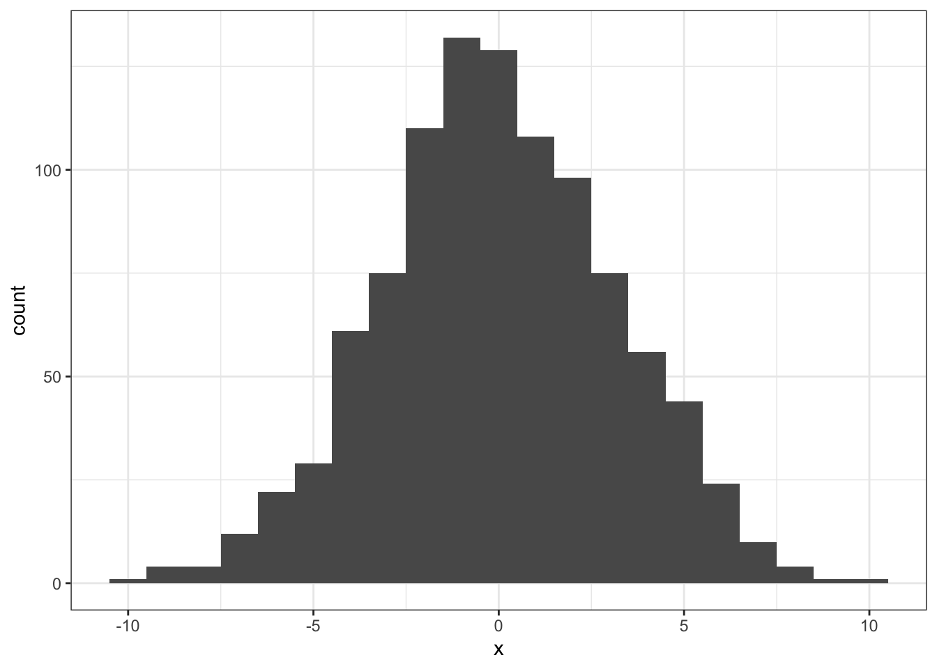

Figure 5.1: The simulated distribution of all possible differences

Return to Task

5.5.1.5 Step 5

Step 5.1 - The logical vector

• This code establishes all the values in nhd that are equal to or greater than the value in d_orig
• It returns all these values as TRUE and all other values as FALSE
• abs() tells the code to ignore the sign of the value (i.e. assumes everything is positive)

lvec = abs(nhd) >= abs(d_orig)

Step 5.2 - Sum up all the TRUE values

• This gives the total number of values greater or equal to d_orig

n_exceeding_orig <- sum(lvec)

Step 5.3 - Calculate the probability

• The probability of obtaining d_orig or greater is calculated by the number of values equal to or greater than d_orig, divided by the full size of nhd (or in other words, its length)

p <- n_exceeding_orig / length(nhd)

• As such the probability of finding a value of \(D_{orig}\) or larger was p = 0.016

To write up the sentence, with inline coding you would write:

• The difference between Group A and Group B (M = `r round(d_orig, 2)`) was found to be have a probability of p = `r p`. This means that the original mean difference was significant and the null hypothesis is rejected.

Which when knitted would produce:

• The difference between Group A and Group B (M = -7.39) was found to be have a probability of p = 0.016. This means that the original mean difference was significant and the null hypothesis is rejected.

Return to Task

Chapter Complete!

5.6 Additional Material

Below is some additional material that might help you understand permutations a bit more and some additional ideas.

More on pivot_wider()

Much in the same way that pivot_longer() has become the new go-to function for gathering data, replacing the gather() function that many struggled with, pivot_wider() is likewise a new kid on the block.

Prior to using pivot_wider(), this book used the very confusing spread() function to change data from long format to wide format - i.e. splitting low columns into more shorter columns. spread() was an interesting function that somehow always managed to confuse people and it seemed that getting it to work was largely chance - pivot_wider() was introduced to reduce these issues and as you saw inclass it works similar to pivot_longer() in that it requires clear statement of names_from and values_from.

pivot_wider() should make spreading data wider a lot easier and as such we have aimed to replace every occurrence of it in this book. However, as before, we are still human and mistakes happen. Also, you will still see it being used in codes that you find on things like StackOverflow etc, so below is a very brief example that mimics the InClass activity, showing how spread() works. For ease, we would always recommend using pivot_wider().

The spread() function

This example mimics Skill 4 (Section 5.2.4) of the Preclass Activity where we are splitting the data in my_data_means - shown below:

• Remember the values will be different from the PreClass because we are using a function that creates a set of random numbers each time, rnorm()

group	m
A	19.63478
B	-19.78001

In order to split the table so that we have one column for Group A and another columns for Group B, we would use the below code. The spread function (?spread) splits the data in column m by the information, i.e. labels, in column group and puts the data into separate columns.

my_data_means %>%
  spread(group, m)

A	B
19.63478	-19.78001

So the spread() function is not that different from using pivot_wider() but the inclusion of names_from and values_from really does make using pivot_wider() a lot clearer.

The rest of the actions in that step of the Activity would follow as in the PreClass Activity - adding a mutate() as shown below:

my_data_means %>%
  spread(group, m) %>%
  mutate(diff = A - B) 

More on simulating your own data

Often we get asked for data to allow people to practice their hand calculations. One of the reasons for this chapter is to show people how to simulate their own data and to give them the functions to do so. We are going to use a chi-square test to show you, in a bit more concrete fashion, how you might go about this. We don’t really cover much about chi-squares in this book so it is a nice addition.

So let’s say we have run an observation test with two groups (A and B) and we ask them the classic “Huey Lewis & the News” question, “Do you believe in love?” giving them three response options, Yes, No, Unsure. Let’s say that we run 50 people in each group as well. Putting that altogether we will end up with a cross-tabulation table that is 2 rows by 3 columns, with each row adding up to 50.

Using everything we have learnt in this Chapter here is how we might simulate that data:

• Going to need at least tidyverse

library(tidyverse)

• The below code is how we might created a tibble (my_chi_data) where you have two columns:
  • Groups showing whether participants are in Group A or B
  • Responses showing the simulated response for that participant

We won’t walk you through this code as you should know enough from Chapters 4 & 5 to follow it and edit it, but if you really struggle, get in touch

my_chi_data <- tibble(Groups = rep(c("A","B"),        # Names of your Groups
                               times = c(50, 50)),    # Participants per Group
                  Responses = sample(c("Yes",         # Response Options to Sample
                                       "No", 
                                       "Unsure"),     
                                     size = 50 + 50,  # Total number of responses
                                     replace = TRUE)) # with replacement

• If you wanted to save your data as a .csv file for later use or to send to a colleague, you could use:

write_csv(my_chi_data, "my_data.csv")

• Or with a bit of data wrangling, you can convert my_chi_data into a cross-tabulation table that would look like as follows:
  • Again this wouldn’t use any new functions
  • group_by() %>% count() %>% pivot_wider()
  • group by both columns as you want to count how many times each response was used by each group.

Table 5.2: Cross-Tabulation Table of Simulated Data for learning about chi-squares

Groups	No	Unsure	Yes	Total
A	17	18	15	50
B	18	14	18	50

More on Permutations - a blog

There is a lot in this chapter and some find all the different components quite tricky. As such, this is a very paired down version of the crux of the chapter to see if removing all the blurb, keeping it to just the essential, helps.

The main concept of Null Hypothesis Significance Testing (NHST) is that you are testing that there is no significant difference between two values - let’s say two means for the moment. The null hypothesis states that there is no meaningful difference between the two groups of interest. And as such, any test that you do on the difference between the means of those two groups is trying to determine the probability of finding a difference of the size you found, or larger, in your experiment, if there is actually no real difference between the two groups.

In the InClass activity we have our two groups, A and B, and we calculated the difference between the means of those two groups to be \(D_{orig}\) = -7.39. Putting that in terms of the Null Hypothesis (\(H_{0}\)) we are asking what is the probability of finding a difference between means of -7.39 (or larger) if there is no real difference between our two groups.

In order to test the above question (our null hypothesis) we need to compare our original difference against a distribution of possible differences to see how likely the original difference is in that distribution - remember, for example, extreme values are in the tails of the Normal Distribution.

As we don’t know where our data comes from we don’t really know what distribution to check our \(D_{orig}\) against. In that situation we can create a distribution based on the values we have already collected using the permutation test we talked about InClass. Basically, in this test, we shuffle which group people belonged to (A or B) and then calculate the difference between these shuffled groups. And we do that 1000 times or more to create a distribution.

The reason we are allowed to shuffle whether people were in group A or B is because we are deliberately wanting to test if the group people were originally in drives the difference we see. If the original grouping of participants is important then the original difference (\(D_{orig}\)) will be an extreme value on the distribution we create. If the group people were originally in isn’t important, then the original difference (\(D_{orig}\)) will not be an extreme value in the distribution; it will be a common value.

Here again is the distribution we simulated using the permutation test described InClass and above:

ggplot(tibble(x = nhd), aes(x)) + geom_histogram(binwidth = 1)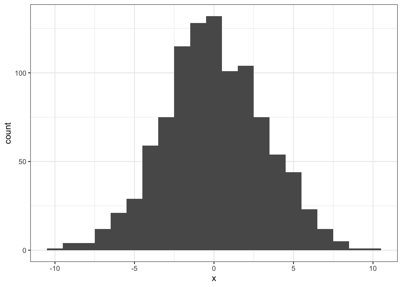

Figure 5.2: The simulated distribution of all possible differences

Now lets highlight the areas in this distribution where the values in the distribution are equal to or larger than our \(D_{orig}\) value - these are the red areas. The blue areas are those where the values in the distribution are smaller than our \(D_{orig}\) value. We have changed the binwidth of the plot a little from above to help see the different areas clearly.

## Warning: `guides(<scale> = FALSE)` is deprecated. Please use `guides(<scale> =
## "none")` instead.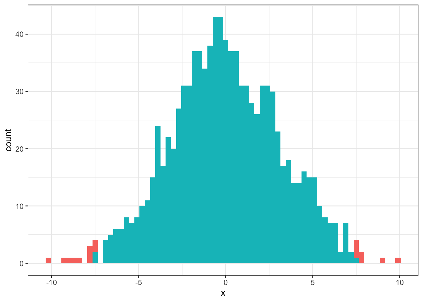

Figure 5.3: The simulated distribution of all possible differences. Red areas show values greater than or equal to the original difference. Blue areas show values smaller than the original difference.

Going back to what we said about Null Hypothesis Significance Testing, the question is what is the probability of finding the original difference (\(D_{orig}\)) if there is no real effect of being in either Group A or Group B. As you can see from the plot, there are very few areas on the distribution where the values are greater than or equal to the original difference - i.e. \(D_{orig}\) is an unlikely difference to obtain if there was really no difference between the two groups. From the InClass you will recall that the probability of finding a difference greater than or equal to \(D_{orig}\) if there was no difference between the two groups was p = 0.017. This is below the standard cut-off we use in Psychology, \(p <= .05\). As such we would reject our null hypothesis and suggest that there is a significant difference between the two groups.

Hopefully this gives a bit more insight to the InClass activities but feel free to post any questions on the forums for discussion or ask a member of staff.

End of Additional Material!